Introduction to Scientific Machine Learning through Physics-Informed Neural Networks
Chris Rackauckas
September 8th, 2020
Youtube Video Link Part 1
Youtube Video Link Part 2
Here we will start to dig into what scientific machine learning is all about by looking at physics-informed neural networks. Let's start by understanding what neural networks really are, why they are used, and what kinds of problems they solve, and then we will use this understanding of a neural network to see how to solve ordinary differential equations with neural networks. For there, we will use this method to regularize neural networks with physical equations, the aforementioned physics-informed neural network, and see how to define neural network architectures that satisfy physical constraints to improve the training process.
Getting Started with Machine Learning: Adding Lux
To add Lux.jl we would do:
]add Lux Optimisers Enzyme ComponentArrays Random
To then use the package we will then use the using command:
using Lux, Optimisers, Enzyme, ComponentArrays, Random
If you prefer to namespace all commands (like is normally done in Python, i.e. Enzyme.autodiff instead of autodiff), you can use the command:
import Lux
Note that the installation and precompilation of these packages will occur at the add and first using phases, so they may take awhile (subsequent uses will utilize the precompiled form and take a lot less time!)
What is a Neural Network?
A neural network is a function:
\[ \text{NN}(x) = W_3\sigma_2(W_2\sigma_1(W_1x + b_1) + b_2) + b_3 \]
where we can change the number of layers ((W_i,b_i)) as necessary. Let's assume we want to approximate some $R^{10} \rightarrow R^5$ function. To do this we need to make sure that we start with 10 inputs and arrive at 5 outputs. If we want a bigger middle layer for example, we can do something like (10,32,32,5). Size changing occurs at the site of the matrix multiplication, which means that we want a 32x10 matrix, then a 32x32 matrix, and finally a 5x32 matrix. This neural network would look like:
W = [randn(32,10),randn(32,32),randn(5,32)]
b = [zeros(32),zeros(32),zeros(5)]
3-element Vector{Vector{Float64}}:
 [0.0, 0.0, 0.0, 0.0, 0.0, 0.0, 0.0, 0.0, 0.0, 0.0  …  0.0, 0.0, 0.0, 0.0,
0.0, 0.0, 0.0, 0.0, 0.0, 0.0]
 [0.0, 0.0, 0.0, 0.0, 0.0, 0.0, 0.0, 0.0, 0.0, 0.0  …  0.0, 0.0, 0.0, 0.0,
0.0, 0.0, 0.0, 0.0, 0.0, 0.0]
 [0.0, 0.0, 0.0, 0.0, 0.0]
simpleNN(x) = W[3]*tanh.(W[2]*tanh.(W[1]*x + b[1]) + b[2]) + b[3]
simpleNN(rand(10))
5-element Vector{Float64}:
  8.186523453521913
  4.023128123115727
  0.7139850661390896
 -6.399990596261691
 -2.8675414967709485
This is our direct definition of a neural network. Notice that we choose to use tanh as our activation function between the layers.
Defining Neural Networks with Lux.jl
One of the main deep learning libraries in Julia is Lux.jl. Lux is an interesting library for scientific machine learning because it is built on top of language-wide automatic differentiation libraries, giving rise to a programming paradigm known as differentiable programming, which means that one can write a program in a manner that it has easily accessible fast derivatives. However, due to being built on a differentiable programming base, the underlying functionality is simply standard Julia code,
To learn how to use the library, consult the documentation. A Google search will bring up the Lux.jl Github repository. From there, the blue link on the README brings you to the package documentation. This is common through Julia so it's a good habit to learn!
In the documentation you will find that the way a neural network is defined is through a Chain of layers. A Dense layer is the kind we defined above, which is given by an input size, an output size, and an activation function. For example, the following recreates the neural network that we had above:
using Lux, Optimisers, Enzyme, ComponentArrays, Random
NN2 = Chain(Dense(10 => 32,tanh),
           Dense(32 => 32,tanh),
           Dense(32 => 5))
ps, st = Lux.setup(Xoshiro(0), NN2)
NN2(rand(Float32, 10), ps, st)[1]
5-element Vector{Float32}:
 -0.31810096
  1.5477026
 -0.6857167
 -0.31069303
 -0.23813409
Notice that Lux.jl as a library is written in pure Julia, which means that every piece of this syntax is just sugar over some Julia code that we can specialize ourselves (this is the advantage of having a language fast enough for the implementation of the library and the use of the library!)
For example, the activation function is just a scalar Julia function. If we wanted to replace it by something like the quadratic function, we can just use an anonymous function to define the scalar function we would like to use:
NN3 = Chain(Dense(10 => 32,x->x^2),
            Dense(32 => 32,x->max(0,x)),
            Dense(32 => 5))
ps, st = Lux.setup(Xoshiro(0), NN3)
NN3(rand(Float32, 10), ps, st)[1]
5-element Vector{Float32}:
 -0.08225827
  0.48074442
  0.12884226
 -0.8241533
  0.22657253
The second activation function there is what's known as a relu. A relu can be good to use because it's an exceptionally fast operation and satisfies a form of the universal approximation theorem (UAT). However, a downside is that its derivative is not continuous, which could impact the numerical properties of some algorithms, and thus it's widely used throughout standard machine learning but we'll see reasons why it may be disadvantageous in some cases in scientific machine learning.
Digging into the Construction of a Neural Network Library
Again, as mentioned before, this neural network NN2 is simply a function:
simpleNN(x) = W[3]*tanh.(W[2]*tanh.(W[1]*x + b[1]) + b[2]) + b[3]
simpleNN (generic function with 1 method)
Let's dig into the library and see how that's represented and really understand the construction of a deep learning library. First, let's figure out where Dense comes from and what it does.
using InteractiveUtils @which Dense(10 => 32,tanh)Dense(mapping::Pair{<:Union{Integer, Static.StaticInteger}, <:Union{Integer, Static.StaticInteger}}, activation; kwargs...) in Lux at /home/runner/.julia/packages/Lux/ZSmgp/src/layers/basic.jl:327
If we go to that spot of the code, we find the following:
struct Dense{F, M<:AbstractMatrix, B}
  weight::M
  bias::B
  σ::F
  function Dense(W::M, bias = true, σ::F = identity) where {M<:AbstractMatrix, F}
    b = create_bias(W, bias, size(W,1))
    new{F,M,typeof(b)}(W, b, σ)
  end
end

function Dense((in, out)::Pair{<:Integer, <:Integer}, σ = identity;
               init = glorot_uniform, bias = true)
  Dense(init(out, in), bias, σ)
end
First, Dense defines a struct in Julia. This struct just holds a weight matrix W, a bias vector b, and an activation function σ. It also defines an inner constructor that ensures that a created Dense object will have the desired properties and types for its fields. The function called Dense that is defined next, outside the struct, is what's known as an outer constructor which provides a more convenient way to create a Dense object. If you give it a Pair of integers (and optionally an activation function which defaults to identity), then what it will do is take random initial W and b matrices (according to the glorot_uniform distribution for W and zeros for b), and then it will build the type with those matrices.
The next portion might be new. We give it here in the simpler form it has in Lux, which makes the parameters and state explicit:
function (a::Dense)(x::AbstractArray, ps, st)
  W, b, σ = ps.weight, ps.bias, a.activation
  σ.(W*x .+ b), st
end
This defines what is known as a callable struct, or a functor. It defines the dispatch for how calls work on the struct. As a quick demonstration, let's define a type MyCallableStruct with a field x, and then make instances of A be the function x+y:
struct MyCallableStruct
  x
end

(a::MyCallableStruct)(y) = a.x+y
a = MyCallableStruct(2)
a(3)
5
If you're familiar with object-oriented programming, this is similar to using an object in a way that references the self, though it's a bit more general due to allowing dispatching, i.e. this can then dependent on the input types as well.
So let's look at Dense with this in mind:
function (a::Dense)(x::AbstractArray)
  W, b, σ = a.W, a.b, a.σ
  σ.(W*x .+ b)
end
This means that Dense is a function that takes in an x and computes σ.(W*x.+b), which is precisely how we defined the layer before! To see that this is just a function, let's call it directly:
denselayer_f = Dense(32 => 32,tanh)
ps, st = Lux.setup(Xoshiro(0), denselayer_f)
denselayer_f(rand(Float32, 32), ps, st)[1]
32-element Vector{Float32}:
 -0.27123606
 -0.09683947
  0.31678876
  0.051858135
  0.4824273
  0.051968176
  0.8487753
 -0.88714886
 -0.34205386
  0.8744724
  ⋮
 -0.0071185906
 -0.84099656
 -0.9160302
 -0.30945918
  0.96569437
  0.2973192
 -0.9151436
  0.6872205
  0.40967488
So okay, Dense objects are just functions that have weight and bias matrices inside of them. Now what does Chain do?
@which Chain(1,2,3)Chain(xs...; name) in Lux at /home/runner/.julia/packages/Lux/ZSmgp/src/layers/containers.jl:542
Again, for our explanations here we will look at the slightly simpler code from an earlier version of the Flux package:
struct Chain{T<:Tuple}
  layers::T
  Chain(xs...) = new{typeof(xs)}(xs)
end

applychain(::Tuple{}, x) = x
applychain(fs::Tuple, x) = applychain(tail(fs), first(fs)(x))

(c::Chain)(x) = applychain(c.layers, x)
Let's now dig into this. The ... is known that the slurp operator, which allows for "slurping up" multiple arguments into a single object xs. For example:
slurper(xs...) = @show xs
slurper(1,2,3,4,5)
xs = (1, 2, 3, 4, 5)
(1, 2, 3, 4, 5)
We see that slurps the inputs up into a Tuple, which is an immutable data store. (Note: Tuples are stack-allocated if inferred and is the internal data store of the compiler itself, and compiler inference can know exactly the size and the type of each individual object, so this does not have an overhead if fully inferred).
The function Chain(xs...) = new{typeof(xs)}(xs) is an inner constructor which builds a new instance of Chain where layers is a tuple of the inputs. This means that in our case where we put a bunch of Dense inside of there, layers is a tuple of functions. What does Chain do? Let's look at its call:
(c::Chain)(x) = applychain(c.layers, x)
This takes the tuple of functions and then does applychain on it.
applychain(::Tuple{}, x) = x
applychain(fs::Tuple, x) = applychain(tail(fs), first(fs)(x))
applychain is a recursive function which applies the first element of the tuple onto x, then it calls applychain to call the second function onto x, repeatedly until there are no more functions in which case it returns x. This means that applychain is simply doing h(g(f(x))) on the tuple of functions (f,g,h)! We can thus see that this library function is exactly equivalent to the neural network we defined by hand, just put together in a different form to give a nice user interface.
Detail: Recursion?
But there's one more detail... why recursion? If you define a function, look at its type:
ff(x,y) = 2x+y
typeof(ff)
typeof(ff) (singleton type of function ff, subtype of Function)
Notice that its type is simply typeof(ff) which is unique to the function, i.e. every single function is its own struct. In fact, given what we just learned, it wouldn't be a surprise to learn that is exactly what a function is in Julia! A function definition lowers at the parser level to something like:
struct ff2 <: Function end
(_::ff2)(x,y) = 2x + y
const ff = ff2()
This means that the primitive operation here that everything really comes down to is calls on structs. Why is this done with unique singleton types? (Singleton types are types where every instance is equivalent). Well, if we want the compiler to be able to optimize with respect to which function we are handling inside of another function, then we need "what function we are dealing with" as compile-time information, which necessitates being type information.
Tuples are covariant and heterogeneously typed with a parameter per internal object. For example:
tup = (1.0,1,"1")
typeof(tup)
Tuple{Float64, Int64, String}
This means that it is possible to infer outputs of a tuple even if it's heterogeneously typed by making good use of constant literals. For example, the expression tup[1] will be inferred to have the output Float64. However, note that if i is not a compile-time constant, then tup[i] cannot be inferred since, given what the compiler knows, the output could be either a Float64, an Int64, or a String.
So now let's think back to our tuple of functions. By what we described before, tup = (f,g,h) is going to have a different type for each of the functions and thus could not specialize on the inputs if we used tup[i]. Therefore:
for i in 1:length(tup)
  x = tup[i](x)
end
would be slow (if the function call cost is small compared to the dispatch cost of about 100ns. This is not always the case, but should be considered in many instances!). So how can you get around it? Well, if everything was constant literals then this would specialize:
tup[3](tup[2](tup[1](x)))
would fully specialize and infer, and the compiler would have full knowledge of the entire call chain as if it were written out as straightline code. Now if we look at the recursion again:
applychain(::Tuple{}, x) = x
applychain(fs::Tuple, x) = applychain(tail(fs), first(fs)(x))
we see that, at compile-time, we know that typeof((f,g,h)) = Tuple{typeof(f),typeof(g),typeof(h)}, and so we know that the first first(fs) will be f, and can specialize on this. We know then that tail(fs) has to be the (g,h) and so then we recurse and know that g is first and ... This means that this scheme is equivalent to have written out xs[3](xs[2](xs[1](x))) and is thus generating code perfectly specialized to the order and amount of functions we had put into the Chain. This kind of abstraction, an abstraction where all of the overhead compiles away, is known as a zero-cost abstraction.
(Note that technically, there is a cost since the compiler has to unravel this chain of events.)
Training Neural Networks
Now let's get into training neural networks. "Training" a neural network is simply the process of finding weights that minimize a loss function. For example, let's say we wanted to make our neural network be the constant function 1 for any input $x \in [0,1]^{10}$. We can then write the loss function:
NN = Chain(Dense(10 => 32,tanh),
           Dense(32 => 32,tanh),
           Dense(32 => 5))
ps, st = Lux.setup(Xoshiro(0), NN)
loss(p) = sum(abs2,sum(abs2,NN(rand(Float32, 10), p, st)[1] .- 1f0) for i in 1:100)
loss(ps)
4123.6445f0
This loss function takes 100 random points in $[0,1]^{10}$ and then computes the output of the neural network minus 1 on each of the values, and sums up the squared values (abs2). Why the squared values? This means that every computed loss value is positive, and so we know that by decreasing the loss this means that, on average our neural network outputs are closer to 1. What are the weights? Since we're using parameter-explicit layers, the weights are inside the ps NamedTuple, which we can inspect:
ps.layer_1.weight # The W matrix of the first layer
32×10 Matrix{Float32}:
 -0.80586      0.67257     0.567036   …  -0.663563    0.801368   -0.619269
 -0.0817231   -0.703158   -0.16772        0.566447    0.55349     0.0353284
  0.750269    -0.071096   -0.0959973      0.551216   -0.862721   -0.432586
  0.0869827    0.885142    0.049274       0.393051   -0.739261   -0.461512
  0.337964     0.775234   -0.698201      -0.0701262   0.630592    0.27304
  0.499073     0.421305   -0.675613   …  -0.408729   -0.714096    0.668322
 -0.707128    -0.217894   -0.374307      -0.819325    0.0688568   0.212683
  0.804394    -0.698652   -0.866057      -0.270632   -0.529147    0.791532
 -0.161699    -0.511234    0.129489      -0.106268    0.445029   -0.795891
 -0.858742     0.326405    0.803168      -0.86848    -0.135339    0.202614
  ⋮                                   ⋱
 -0.492697     0.0277226   0.472546       0.552228   -0.513784   -0.700641
  0.497144    -0.553627    0.332054       0.555452   -0.730213   -0.850277
  0.23964      0.227052    0.771982   …   0.322942    0.63799    -0.0977781
 -0.295106     0.591531    0.473602       0.695275    0.795155   -0.453172
 -0.736409     0.280706   -0.474823      -0.0934138   0.406972    0.266934
  0.578627    -0.816865    0.344601       0.143064    0.444296   -0.458468
  0.361515     0.745637    0.487035      -0.0466465   0.720389   -0.417548
  8.05288f-6  -0.523924    0.825575   …   0.13543     0.814132    0.056694
 -0.0543024    0.128128   -0.22217       -0.672352    0.197776   -0.580463
Now let's train the neural network by finding the optimal parameters which cause it to be the constant 1 function. We use Lux.Training.TrainState and Lux.Training.single_train_step! to compute the gradients and update the parameters in a loop:
tstate = Lux.Training.TrainState(NN, ps, st, Adam(0.1f0))

function opt_loss(model, p, st, x)
   pred, st_new = model(x, p, st)
   return sum(abs2, pred .- 1f0), st_new, ()
end

for epoch in 1:10000
    global tstate
    x = rand(Float32, 10, 128)
    _, _, _, tstate = Lux.Training.single_train_step!(
        AutoEnzyme(), opt_loss, x, tstate
    )
end
Now let's check the loss:
loss(tstate.parameters)
2.3714845f-6
This means that NN(x, p, st)[1] is now a very good function approximator to f(x) = ones(5)!
So Why Machine Learning? Why Neural Networks?
All we did was find parameters that made NN(x) act like a function f(x). How does that relate to machine learning? Well, in any case where one is acting on data (x,y), the idea is to assume that there exists some underlying mathematical model f(x) = y. If we had perfect knowledge of what f is, then from only the information of x we can then predict what y would be. The inference problem is to then figure out what function f should be. Therefore, machine learning on data is simply this problem of finding an approximator to some unknown function!
So why neural networks? Neural networks satisfy two properties. The first of which is known as the Universal Approximation Theorem (UAT), which in simple non-mathematical language means that, for any ϵ of accuracy, if your neural network is large enough (has enough layers, the weight matrices are large enough), then it can approximate any (nice) function f within that ϵ. Therefore, we can reduce the problem of finding missing functions, the problem of machine learning, to a problem of finding the weights of neural networks, which is a well-defined mathematical optimization problem.
Why neural networks specifically? That's a fairly good question, since there are many other functions with this property. For example, you will have learned from analysis that $a_0 + a_1 x + a_2 x^2 + \ldots$ arbitrary polynomials can be used to approximate any analytic function (this is the Taylor series). Similarly, a Fourier series
\[ f(x) = a_0 + \sum_k b_k \cos(kx) + c_k \sin(kx) \]
can approximate any continuous function f (and discontinuous functions also can have convergence, etc. these are the details of a harmonic analysis course).
That's all for one dimension. How about two dimensional functions? It turns out it's not difficult to prove that tensor products of universal approximators will give higher dimensional universal approximators. So for example, tensoring together two polynomials:
\[ a_0 + a_1 x + a_2 y + a_3 x y + a_4 x^2 y + a_5 x y^2 + a_6 x^2 y^2 + \ldots \]
will give a two-dimensional function approximator. But notice how we have to resolve every combination of terms. This means that if we used n coefficients in each dimension d, the total number of coefficients to build a d-dimensional universal approximator from one-dimensional objects would need $n^d$ coefficients. This exponential growth is known as the curse of dimensionality.
The second property of neural networks that makes them applicable to machine learning is that they overcome the curse of dimensionality. The proofs in this area can be a little difficult to parse, but what they boil down to is proving in many cases that the growth of neural networks to sufficiently approximate a d-dimensional function grows as a polynomial of d, rather than exponential. This means that there's some dimensional cutoff where for $d>cutoff$ it is more efficient to use a neural network. This can be problem-specific, but generally it tends to be the case at least by 8 or 10 dimensions.
Neural networks have a few other properties to consider as well:
The assumptions of the neural network can be encoded into the neural architectures. A neural network where the last layer has an activation function
x->x^2is a neural network where all outputs are positive. This means that if you want to find a positive function, you can make the optimization easier by enforcing this constraint. A lot of other constraints can be enforced, liketanhactivation functions can make the neural network be a smooth (all derivatives finite) function, or other activations can cause finite numbers of learnable discontinuities.Generating higher dimensional forms from one dimensional forms does not have good symmetry. For example, the two-dimensional tensor Fourier basis does not have a good way to represent $sin(xy)$. This property of the approximator is called (non)isotropy and more detail can be found in this wonderful talk about function approximation for multidimensional integration (cubature). Neural networks are naturally not aligned to a basis.
Neural networks are "easy" to compute. There's good software for them, GPU-acceleration, and all other kinds of tooling that make them particularly simple to use.
There are proofs that in many scenarios for neural networks the local minima are the global minima, meaning that local optimization is sufficient for training a neural network. Global optimization (which we will cover later in the course) is much more expensive than local methods like gradient descent, and thus this can be a good property to abuse for faster computation.
From Machine Learning to Scientific Machine Learning: Structure and Science
This understanding of a neural network and their libraries directly bridges to the understanding of scientific machine learning and the computation done in the field. In scientific machine learning, neural networks and machine learning are used as the basis to solve problems in scientific computing. Scientific computing, as a discipline also known as Computational Science, is a field of study which focuses on scientific simulation, using tools such as differential equations to investigate physical, biological, and other phenomena.
What we wish to do in scientific machine learning is use these properties of neural networks to improve the way that we investigate our scientific models.
Aside: Why Differential Equations?
Why do differential equations come up so often in as the model in the scientific context? This is a deep question with quite a simple answer. Essentially, all scientific experiments always have to test how things change. For example, you take a system now, you change it, and your measurement is how the changes you made caused changes in the system. This boils down to gather information about how, for some arbitrary system $y = f(x)$, how $\Delta x$ is related to $\Delta y$. Thus what you learn from scientific experiments, what is codified as scientific laws, is not "the answer", but the answer to how things change. This process of writing down equations by describing how they change precisely gives differential equations.
Solving ODEs with Neural Networks: The Physics-Informed Neural Network
Now let's get to our first true SciML application: solving ordinary differential equations with neural networks. The process of solving a differential equation with a neural network, or using a differential equation as a regularizer in the loss function, is known as a physics-informed neural network, since this allows for physical equations to guide the training of the neural network in circumstances where data might be lacking.
Background: A Method for Solving Ordinary Differential Equations with Neural Networks
This is a result first due to Lagaris et. al from 1998. The idea is to solve differential equations using neural networks by representing the solution by a neural network and training the resulting network to satisfy the conditions required by the differential equation.
Let's say we want to solve a system of ordinary differential equations
\[ u' = f(u,t) \]
with $t \in [0,1]$ and a known initial condition $u(0)=u_0$. To solve this, we approximate the solution by a neural network:
\[ NN(t) \approx u(t) \]
If $NN(t)$ was the true solution, then it would hold that $NN'(t) = f(NN(t),t)$ for all $t$. Thus we turn this condition into our loss function. This motivates the loss function:
\[ L(p) = \sum_i \left(\frac{dNN(t_i)}{dt} - f(NN(t_i),t_i) \right)^2 \]
The choice of $t_i$ could be done in many ways: it can be random, it can be a grid, etc. Anyways, when this loss function is minimized (gradients computed with standard reverse-mode automatic differentiation), then we have that $\frac{dNN(t_i)}{dt} \approx f(NN(t_i),t_i)$ and thus $NN(t)$ approximately solves the differential equation.
Note that we still have to handle the initial condition. One simple way to do this is to add an initial condition term to the cost function. This would look like:
\[ L(p) = (NN(0) - u_0)^2 + \sum_i \left(\frac{dNN(t_i)}{dt} - f(NN(t_i),t_i) \right)^2 \]
While that would work, it can be more efficient to encode the initial condition into the function itself so that it's trivially satisfied for any possible set of parameters. For example, instead of directly using a neural network, we can use:
\[ g(t) = u_0 + tNN(t) \]
as our solution. Notice that $g(t)$ is thus a universal approximator for all continuous functions such that $g(0)=u_0$ (this is a property one should prove!). Since $g(t)$ will always satisfy the initial condition, we can train $g(t)$ to satisfy the derivative function then it will automatically be a solution to the derivative function. In this sense, we can use the loss function:
\[ L(p) = \sum_i \left(\frac{dg(t_i)}{dt} - f(g(t_i),t_i) \right)^2 \]
where $p$ are the parameters that define $g$, which in turn are the parameters which define the neural network $NN$ that define $g$. Thus this reduces down, once again, to simply finding weights which minimize a loss function!
Coding Up the Method
Now let's implement this method with Lux. Let's define a neural network to be the NN(t) above. To make the problem easier, let's look at the ODE:
\[ u' = \cos 2\pi t \]
and approximate it with the neural network from a scalar to a scalar:
using Lux, Optimisers, Enzyme, ComponentArrays, Random

 # Take in a scalar and transform it into an array
scalar_to_vector(x::Number) = reshape([x], 1, 1)
scalar_to_vector(x::AbstractVector) = reshape(x, 1, length(x))
scalar_to_vector(x::AbstractMatrix) = x

NNODE = Chain(WrappedFunction(scalar_to_vector),
              Dense(1 => 32,tanh),
              Dense(32 => 1))
ps, st = Lux.setup(Xoshiro(0), NNODE)
NNODE(1.0f0, ps, st)[1]
1×1 Matrix{Float32}:
 0.7322487
Instead of directly approximating the neural network, we will use the transformed equation that is forced to satisfy the boundary conditions. Using u0=1.0, we have the function:
struct ModelWrapper{M} <: AbstractLuxWrapperLayer{:model}
    model::M
end

function (m::ModelWrapper)(t, p, st)
    y, st = m.model(t, p, st)
    return scalar_to_vector(t) .* y .+ 1f0, st
end
model = ModelWrapper(NNODE)
ps, st = Lux.setup(Xoshiro(0), model)
model(1.0f0, ps, st)[1]
1×1 Matrix{Float32}:
 1.7322488
as our universal approximator. Thus, for this to be a function that satisfies
\[ g' = \cos 2\pi t \]
we would need that:
using Statistics

function loss(p)
    ϵ = sqrt(eps(Float32))
    t = 0f0:1f-2:1f0
    t_plus_ϵ = t .+ ϵ
    diff = (model(t_plus_ϵ, p, st)[1] .- model(t, p, st)[1]) / ϵ
    return mean(abs2, diff .- cos.(Float32(2π) .* scalar_to_vector(t)))
end
loss (generic function with 1 method)
would be minimized.
tstate = Lux.Training.TrainState(model, ps, st, Descent(0.01f0))

function opt_loss(model, p, st, ts)
    ϵ = sqrt(eps(Float32))
    ts_plus_ϵ = ts .+ ϵ

    y, st = model(ts, p, st)
    y_plus_ϵ, st = model(ts_plus_ϵ, p, st)

    diff = (y_plus_ϵ .- y) ./ ϵ
    return MSELoss()(diff, cos.(Float32(2π) .* ts)), st, (;)
end

for epoch in 1:5000
    global tstate
    _, loss, _, tstate = Lux.Training.single_train_step!(
      AutoEnzyme(), opt_loss, reshape(collect(0f0:1f-2:1f0), 1, :), tstate
    )
    if epoch % 500 == 0 || epoch == 1
        @info "Training" epoch loss
    end
end
How well did this do? Well if we take the integral of both sides of our differential equation, we see it's fairly trivial:
\[ \int g' = g = \int \cos 2\pi t = C + \frac{\sin 2\pi t}{2\pi} \]
where we defined $C = 1$. Let's take a bunch of (input,output) pairs from the neural network and plot it against the analytical solution to the differential equation:
using Plots
t = 0f0:0.001f0:1f0
g(t, p) = model(t, p, tstate.states)[1]
plot(t,vec(g(t, tstate.parameters)),label="NN")
plot!(t,1.0 .+ sin.(2π.*t)/2π, label = "True Solution")

We see that it matches very well, and we can keep improving this fit by increasing the size of the neural network, using more training points, and training for more iterations.
Example: Harmonic Oscillator Informed Training
Using this idea, differential equations encoding physical laws can be utilized inside of loss functions for terms which we have some basis to believe should approximately follow some physical system. Let's investigate this last step by looking at how to inform the training of a neural network using the harmonic oscillator.
Let's assume that we are taking measurements of (position,force) in some real one-dimensional spring pushing and pulling against a wall.
But instead of the simple spring, let's assume we had a more complex spring, for example, let's say $F(x) = -kx + 0.1sin(x)$ where this extra term is due to some deformities in the metal (assume mass=1). Then by Newton's law of motion we have a second order ordinary differential equation:
\[ x'' = -kx + 0.1 \sin(x) \]
We can use the DifferentialEquations.jl package to solve this differential equation and see what this system looks like:
using DifferentialEquations
k = 1.0
force(dx,x,k,t) = -k*x + 0.1sin(x)
prob = SecondOrderODEProblem(force,1.0,0.0,(0.0,10.0),k)
sol = solve(prob)
plot(sol,label=["Velocity" "Position"])

Don't worry if you don't understand this syntax yet: we will go over differential equation solvers and DifferentialEquations.jl in a later lecture.
Let's say we want to learn how to predict the force applied on the spring at each point in space, $F(x)$. We want to learn a function, so this is the job for machine learning! However, we only have 6 measurements, which includes the information about (position,velocity,force) at evenly spaced times:
plot_t = 0:0.01:10
data_plot = sol(plot_t)
positions_plot = [state[2] for state in data_plot.u]
force_plot = [force(state[1],state[2],k,t) for state in data_plot.u]

# Generate the dataset
t = 0:3.3:10
dataset = sol(t)
position_data = [state[2] for state in sol(t).u]
force_data = [force(state[1],state[2],k,t) for state in sol(t).u]

plot(plot_t,force_plot,xlabel="t",label="True Force")
scatter!(t,force_data,label="Force Measurements")

Can we train a neural network to approximate the expected force at any location for this spring? To see whether this is possible with a standard neural network, let's just do it. Let's define a neural network to be $F(x)$ and see if we can learn the force function!
NNForce = Chain(WrappedFunction(scalar_to_vector),
           Dense(1 => 32,tanh),
           Dense(32 => 1))
ps2, st2 = Lux.setup(Xoshiro(0), NNForce)
((layer_1 = NamedTuple(), layer_2 = (weight = Float32[-2.548353; -0.2584312
; … ; 2.5465439f-5; -0.17171931;;], bias = Float32[0.35222304, -0.6797136,
0.9589201, 0.0022716522, -0.738904, -0.96251273, -0.29784334, 0.72036564, 0
.47573137, 0.31127203  …  -0.94381857, 0.16997182, 0.63449347, 0.27660978,
0.7366687, 0.5446098, -0.30952382, 0.87671924, -0.9684769, 0.63429606]), la
yer_3 = (weight = Float32[0.2037279 0.10215899 … 0.18105792 -0.14819482], b
ias = Float32[0.076488815])), (layer_1 = NamedTuple(), layer_2 = NamedTuple
(), layer_3 = NamedTuple()))
Now our loss function will be to match the force at the (position,force) pairs in the dataset:
function loss_force(p)
    pos = Float32.(position_data)
    force = scalar_to_vector(Float32.(force_data))
    return MSELoss()(NNForce(pos, p, st2)[1], force)
end

loss_force(ps2)
0.400833f0
Our random parameters do not do so well, so let's train!
tstate2 = Lux.Training.TrainState(NNForce, ps2, st2, Descent(0.01f0))

function opt_loss_force(model, p, s, (position_data, force_data))
    pos = Float32.(position_data)
    force = scalar_to_vector(Float32.(force_data))
    force_pred, st = model(pos, p, s)
    return MSELoss()(force_pred, force), st, ()
end

for epoch in 1:5000
    global tstate2
    _, loss_val, _, tstate2 = Lux.Training.single_train_step!(
        AutoEnzyme(), opt_loss_force, (position_data, force_data), tstate2
    )
    if epoch % 500 == 0
        @info "Training" epoch loss_val
    end
end
The neural network almost exactly matched the dataset, but how well did it actually learn the real force function? Let's plot it to see:
learned_force_plot = vec(
    NNForce(Float32.(positions_plot), tstate2.parameters, tstate2.states)[1]
)

plot(plot_t,force_plot,xlabel="t",label="True Force")
plot!(plot_t,learned_force_plot,label="Predicted Force")
scatter!(t,force_data,label="Force Measurements")

Ouch. The problem is that a neural network can approximate any function, so it approximated a function that fits the data, but not the correct function. We somehow need to have more data... but where can we get more data?
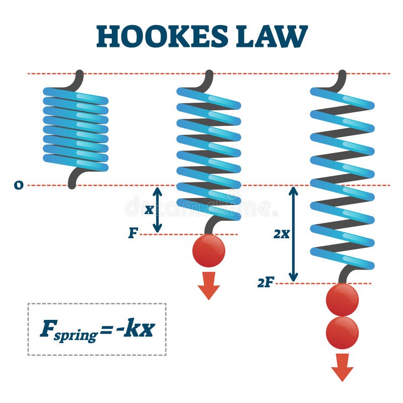
Well, even a first year undergrad in physics will know Hooke's law, which is that the idealized spring should satisfy $F(x) = -kx$. This is a decent assumption for the evolution of the system:
force2(dx,x,k,t) = -k*x
prob_simplified = SecondOrderODEProblem(force2,1.0,0.0,(0.0,10.0),k)
sol_simplified = solve(prob_simplified)
plot(sol,label=["Velocity" "Position"])
plot!(sol_simplified,label=["Velocity Simplified" "Position Simplified"])

While it's not quite correct, and it definitely drifts near the end, it should be a useful non-data assumption that we can add to improve the fitting. So, assuming we know $k$ (this lab you probably have done before!), we can regularize this fitting by having a term that states our neural network should be the solution to the differential equation.
This term looks like what we had done before:
random_positions = Float32[2rand()-1 for i in 1:100] # random values in [-1,1]

function loss_ode(p)
    positions = scalar_to_vector(Float32.(random_positions))
    return MSELoss()(NNForce(positions, p, tstate2.states)[1], Float32.(-k*positions))
end

loss_ode(tstate2.parameters)
0.3167246f0
If this term is zero, then $F(x) = -kx$, which is approximately true. So now let's put these together:
λ = 0.1f0
composed_loss(p) = loss_force(p) + λ*loss_ode(p)
composed_loss (generic function with 1 method)
where $λ$ is some weight factor to control the regularization against the physics assumption. Now we can train the physics-informed neural network:
# Reset train state
tstate2 = Lux.Training.TrainState(NNForce, Lux.setup(Xoshiro(0), NNForce)..., Descent(0.01f0))

function opt_composed_loss(model, p, s, (pos, force, rand_pos))
    loss_force_val, s, _ = opt_loss_force(model, p, s, (pos, force))
    positions = scalar_to_vector(Float32.(rand_pos))
    force_pred, s = model(positions, p, s)
    loss_ode_val = MSELoss()(force_pred, Float32.(-k * positions))
    return (
        loss_force_val + λ * loss_ode_val,
        s,
        (; loss_force=loss_force_val, loss_ode=loss_ode_val)
    )
end

display(composed_loss(tstate2.parameters))
for epoch in 1:5000
    global tstate2
    rand_pos = 2 .* rand(Float32, 100) .- 1
    _, loss, stats, tstate2 = Lux.Training.single_train_step!(
        AutoEnzyme(), opt_composed_loss, (position_data, force_data, rand_pos), tstate2
    )
    if epoch % 500 == 0
        @info "Training" epoch loss stats.loss_force stats.loss_ode
    end
end

learned_force_plot = vec(
    NNForce(Float32.(positions_plot), tstate2.parameters, tstate2.states)[1]
)

plot(plot_t,force_plot,xlabel="t",label="True Force")
plot!(plot_t,learned_force_plot,label="Predicted Force")
scatter!(t,force_data,label="Force Measurements")
0.5182285f0

And there we go: we have used knowledge of physics to help inform our neural network training process!
Conclusion
In this lecture we motivated machine learning not as a process of predicting from data but as a process for learning arbitrary nonlinear functions. Neural networks were just one choice of possible function. We then demonstrated how differential equations could be solved using this function approximation technique and then put together these two domains, solving differential equations and approximating data, into a single process to allow for physical knowledge to be embedded into the training process of a neural network, thus arriving at a physics-informed neural network. This is just one method in scientific machine learning which we will be exploring in more detail, demonstrating how we can utilize scientific knowledge to improve fits and allow for data-efficient machine learning.