The Basics of Single Node Parallel Computing
Chris Rackauckas
September 21st, 2020
Youtube Video Link
Moore's law was the idea that computers double in efficiency at fixed time points, leading to exponentially more computing power over time. This was true for a very long time.

However, sometime in the last decade, computer cores have stopped getting faster.
The technology that promises to keep Moore’s Law going after 2013 is known as extreme ultraviolet (EUV) lithography. It uses light to write a pattern into a chemical layer on top of a silicon wafer, which is then chemically etched into the silicon to make chip components. EUV lithography uses very high energy ultraviolet light rays that are closer to X-rays than visible light. That’s attractive because EUV light has a short wavelength—around 13 nanometers—which allows for making smaller details than the 193-nanometer ultraviolet light used in lithography today. But EUV has proved surprisingly difficult to perfect.
-MIT Technology Review
The answer to the “end of Moore's Law” is Parallel Computing. However, programs need to be specifically designed in order to adequately use parallelism. This lecture will describe at a very high level the forms of parallelism and when they are appropriate. We will then proceed to use shared-memory multithreading to parallelize the simulation of the discrete dynamical system.
Managing Threads
Concurrency vs Parallelism and Green Threads
There is a difference between concurrency and parallelism. In a nutshell:
Concurrency: Interruptability
Parallelism: Independentability
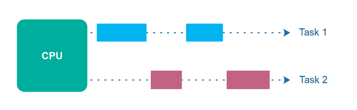
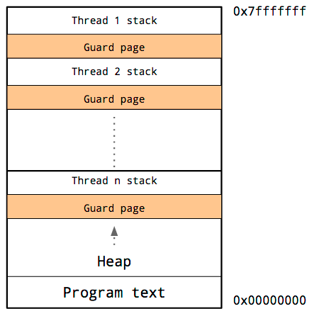
To start thinking about concurrency, we need to distinguish between a process and a thread. A process is discrete running instance of a computer program. It has allocated memory for the program's code, its data, a heap, etc. Each process can have many compute threads. These threads are the unit of execution that needs to be done. On each task is its own stack and a virtual CPU (virtual CPU since it's not the true CPU, since that would require that the task is ON the CPU, which it might not be because the task can be temporarily halted). The kernel of the operating systems then schedules tasks, which runs them. In order to keep the computer running smooth, context switching, i.e. changing the task that is actually running, happens all the time. This is independent of whether tasks are actually scheduled in parallel or not.

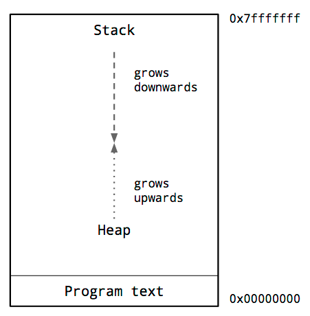
Each thread has its own stack associated with it.
This is an important distinction because many tasks may need to run concurrently but without parallelism. Examples of this are input/output (I/O). For example, in a game you may want to be updating the graphics, but the moment a user clicks you want to handle that event. You do not necessarily need to have these running in parallel, but you need the event handling task to be running concurrently to the processing of the game.

Data handling is the key area of scientific computing where green threads (concurrent non-parallel threads) show up. For data handling, one may need to send a signal that causes a message to start being passed. Alternative hardware take over at that point. This alternative hardware is a processor specific for an I/O bus, like the controller for the SSD, modem, GPU, or Infiniband. It will be polled, then it will execute the command, and give the result. There are two variants:
Non-Blocking vs Blocking: Whether the thread will periodically poll for whether that task is complete, or whether it should wait for the task to complete before doing anything else
Synchronous vs Asynchronous: Whether to execute the operation as initiated by the program or as a response to an event from the kernel.
I/O operations cause a privileged context switch, allowing the task which is handling the I/O to directly be switched to in order to continue actions.
The Main Event Loop
Julia, along with other languages with a runtime (Javascript, Go, etc.) at its core is a single process running an event loop. This event loop is the main thread, and "Julia program" or "script" that one is running is actually ran in a green thread that is controlled by the main event loop. The event loop takes over to look for other work whenever the program hits a yield point. More yield points allows for more aggressive task switching, while it also means more switches to the event loop which suspends the numerical task, i.e. making it slower. Thus yielding shouldn't interrupt the main loop!
This is one area where languages can wildly differ in implementation. Languages structured for lots of I/O and input handling, like Javascript, have yield points at every line (it's an interpreted language and therefore the interpreter can always take control). In Julia, the yield points are minimized. The common yield points are allocations and I/O (println). This means that a tight non-allocating inner loop will not have any yield points and will be a thread that is not interruptible. While this is great for numerical performance, it is something to be aware of.
Side effect: if you run a long tight loop and wish to exit it, you may try Ctrl + C and see that it doesn't work. This is because interrupts are handled by the event loop. The event loop is never re-entered until after your tight numerical loop, and therefore you have the waiting occur. If you hit Ctrl + C multiple times, you will escalate the interruption until the OS takes over and then this is handled by the signal handling of the OS's event loop, which sends a higher level interrupt which Julia handles the moment the safety locks says it's okay (these locks occur during memory allocations to ensure that memory is not corrupted).
Asynchronous Calling Example
This example will become more clear when we get to distributed computing, but for now think of remotecall_fetch as a way to run a command on a different computer. What we want to do is start all of the commands at once, and then wait for all the results before finishing the loop. We will use @async to make the call to remotecall_fetch be non-blocking, i.e. it'll start the job and only poll infrequently to find out when the other machine has completed the job and returned the result. We then add @sync to the loop, which will only continue the loop after all of the green threads have fetched the result. Otherwise, it's possible that a[idx] may not be filled yet, since the thread may not have fetched the result!
@time begin
    a = Vector{Any}(undef,nworkers())
    @sync for (idx, pid) in enumerate(workers())
        @async a[idx] = remotecall_fetch(sleep, pid, 2)
    end
end
The same can be done for writing to the disk. @async is a quick shorthand for spawning a green thread which will handle that I/O operation, and the main event loop will keep switching between them until they are all handled. @sync encodes that the program will not continue until all green threads are handled. This could be done more manually with Task and Channels, which will be something we touch on in the future.
Examples of the Differences
Synchronous = Thread will complete an action
Blocking = Thread will wait until action is completed
Asynchronous + Non-Blocking: I/O
Asynchronous + Blocking: Threaded atomics (demonstrated next lecture)
Synchronous + Blocking: Standard computing,
@syncSynchronous + Non-Blocking: Webservers where an I/O operation can be performed, but one never checks if the operation is completed.
Multithreading
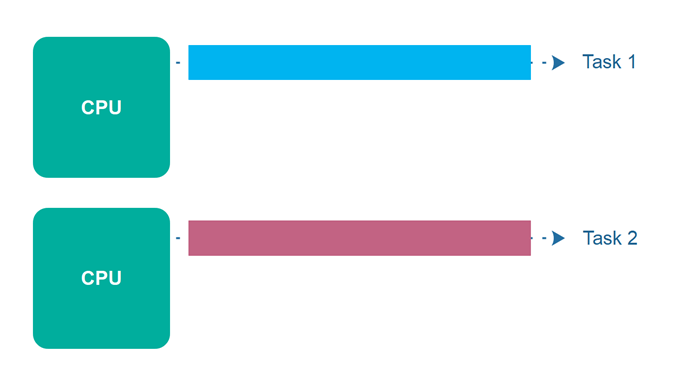
If your threads are independent, then it may make sense to run them in parallel. This is the form of parallelism known as multithreading. To understand the data that is available in a multithreaded setup, let's look at the picture of threads again:
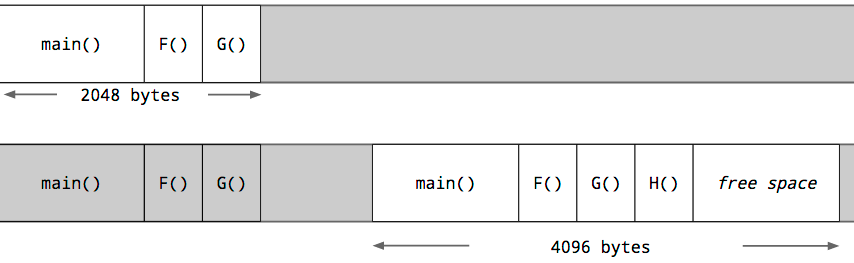
Each thread has its own call stack, but it's the process that holds the heap. This means that dynamically-sized heap allocated objects are shared between threads with no cost, a setup known as shared-memory computing.
Loop-Based Multithreading with @threads
Let's look back at our Lorenz dynamical system from before:
using StaticArrays, BenchmarkTools
function lorenz(u,p)
  α,σ,ρ,β = p
  @inbounds begin
    du1 = u[1] + α*(σ*(u[2]-u[1]))
    du2 = u[2] + α*(u[1]*(ρ-u[3]) - u[2])
    du3 = u[3] + α*(u[1]*u[2] - β*u[3])
  end
  @SVector [du1,du2,du3]
end
function solve_system_save!(u,f,u0,p,n)
  @inbounds u[1] = u0
  @inbounds for i in 1:length(u)-1
    u[i+1] = f(u[i],p)
  end
  u
end
p = (0.02,10.0,28.0,8/3)
u = Vector{typeof(@SVector([1.0,0.0,0.0]))}(undef,1000)
@btime solve_system_save!(u,lorenz,@SVector([1.0,0.0,0.0]),p,1000)
4.759 μs (0 allocations: 0 bytes)
1000-element Vector{SVector{3, Float64}}:
 [1.0, 0.0, 0.0]
 [0.8, 0.56, 0.0]
 [0.752, 0.9968000000000001, 0.008960000000000001]
 [0.80096, 1.3978492416000001, 0.023474005333333336]
 [0.92033784832, 1.8180538219817644, 0.04461448495326095]
 [1.099881043052353, 2.296260732619613, 0.07569952060880669]
 [1.339156980965805, 2.864603692722823, 0.12217448583728006]
 [1.6442463233172087, 3.5539673118971193, 0.19238159391549564]
 [2.026190521033191, 4.397339452147425, 0.2989931959555302]
 [2.5004203072560376, 5.431943011293093, 0.4612438424853632]
 ⋮
 [6.8089180814322185, 0.8987564841782779, 31.6759436385101]
 [5.6268857619814305, 0.3801973723631693, 30.108951163308078]
 [4.577548084057778, 0.13525687944525802, 28.545926978224173]
 [3.6890898431352737, 0.08257160199224252, 27.035860436772758]
 [2.9677861949066675, 0.15205611935372762, 25.600040161309696]
 [2.4046401797960795, 0.2914663505185634, 24.24373008707723]
 [1.9820054139405763, 0.46628657468365653, 22.964748583050085]
 [1.6788616460891923, 0.6565587545689172, 21.758445642263496]
 [1.4744010677851374, 0.8530017039412324, 20.62004063423844]
In order to use multithreading on this code, we need to take a look at the dependency graph and see what items can be calculated independently of each other. Notice that
σ*(u[2]-u[1])
ρ-u[3]
u[1]*u[2]
β*u[3]
are all independent operations, so in theory we could split those off to different threads, move up, etc.
Or we can have three threads:
u[1] + α*(σ*(u[2]-u[1]))
u[2] + α*(u[1]*(ρ-u[3]) - u[2])
u[3] + α*(u[1]*u[2] - β*u[3])
all don't depend on the output of each other, so these tasks can be run in parallel. We can do this by using Julia's Threads.@threads macro which puts each of the computations of a loop in a different thread. The threaded loops do not allow you to return a value, so how do you build up the values for the @SVector?
...?
...?
...?
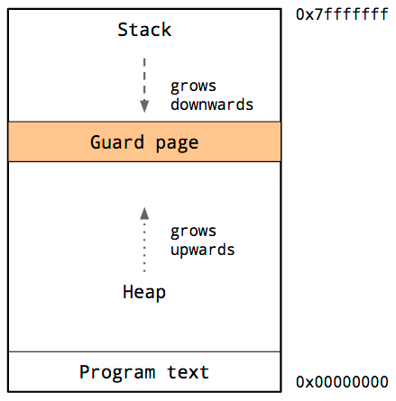
It's not possible! To understand why, let's look at the picture again:
There is a shared heap, but the stacks are thread local. This means that a value cannot be stack allocated in one thread and magically appear when re-entering the main thread: it needs to go on the heap somewhere. But if it needs to go onto the heap, then it makes sense for us to have preallocated its location. But if we want to preallocate du[1], du[2], and du[3], then it makes sense to use the fully non-allocating update form:
function lorenz!(du,u,p)
  α,σ,ρ,β = p
  @inbounds begin
    du[1] = u[1] + α*(σ*(u[2]-u[1]))
    du[2] = u[2] + α*(u[1]*(ρ-u[3]) - u[2])
    du[3] = u[3] + α*(u[1]*u[2] - β*u[3])
  end
end
function solve_system_save_iip!(u,f,u0,p,n)
  @inbounds u[1] = u0
  @inbounds for i in 1:length(u)-1
    f(u[i+1],u[i],p)
  end
  u
end
p = (0.02,10.0,28.0,8/3)
u = [Vector{Float64}(undef,3) for i in 1:1000]
@btime solve_system_save_iip!(u,lorenz!,[1.0,0.0,0.0],p,1000)
7.286 μs (2 allocations: 80 bytes)
1000-element Vector{Vector{Float64}}:
 [1.0, 0.0, 0.0]
 [0.8, 0.56, 0.0]
 [0.752, 0.9968000000000001, 0.008960000000000001]
 [0.80096, 1.3978492416000001, 0.023474005333333336]
 [0.92033784832, 1.8180538219817644, 0.04461448495326095]
 [1.099881043052353, 2.296260732619613, 0.07569952060880669]
 [1.339156980965805, 2.864603692722823, 0.12217448583728006]
 [1.6442463233172087, 3.5539673118971193, 0.19238159391549564]
 [2.026190521033191, 4.397339452147425, 0.2989931959555302]
 [2.5004203072560376, 5.431943011293093, 0.4612438424853632]
 ⋮
 [6.8089180814322185, 0.8987564841782779, 31.6759436385101]
 [5.6268857619814305, 0.3801973723631693, 30.108951163308078]
 [4.577548084057778, 0.13525687944525802, 28.545926978224173]
 [3.6890898431352737, 0.08257160199224252, 27.035860436772758]
 [2.9677861949066675, 0.15205611935372762, 25.600040161309696]
 [2.4046401797960795, 0.2914663505185634, 24.24373008707723]
 [1.9820054139405763, 0.46628657468365653, 22.964748583050085]
 [1.6788616460891923, 0.6565587545689172, 21.758445642263496]
 [1.4744010677851374, 0.8530017039412324, 20.62004063423844]
and now we multithread:
using Base.Threads
function lorenz_mt!(du,u,p)
  α,σ,ρ,β = p
  let du=du, u=u, p=p
    Threads.@threads for i in 1:3
      @inbounds begin
        if i == 1
          du[1] = u[1] + α*(σ*(u[2]-u[1]))
        elseif i == 2
          du[2] = u[2] + α*(u[1]*(ρ-u[3]) - u[2])
        else
          du[3] = u[3] + α*(u[1]*u[2] - β*u[3])
        end
        nothing
      end
    end
  end
  nothing
end
function solve_system_save_iip!(u,f,u0,p,n)
  @inbounds u[1] = u0
  @inbounds for i in 1:length(u)-1
    f(u[i+1],u[i],p)
  end
  u
end
p = (0.02,10.0,28.0,8/3)
u = [Vector{Float64}(undef,3) for i in 1:1000]
@btime solve_system_save_iip!(u,lorenz_mt!,[1.0,0.0,0.0],p,1000);
3.672 ms (21980 allocations: 1.62 MiB)
Parallelism doesn't always make things faster. There are two costs associated with this code. For one, we had to go to the slower heap+mutation version, so its implementation starting point is slower. But secondly, and more importantly, the cost of spinning a new thread is non-negligible. In fact, here we can see that it even needs to make a small allocation for the new context. The total cost is on the order of 50ns: not huge, but something to take note of. So what we've done is taken almost free calculations and made them ~50ns by making each in a different thread, instead of just having it be one thread with one call stack.
The moral of the story is that you need to make sure that there's enough work per thread in order to effectively accelerate a program with parallelism.
Data-Parallel Problems
So not every setup is amenable to parallelism. Dynamical systems are notorious for being quite difficult to parallelize because the dependency of the future time step on the previous time step is clear, meaning that one cannot easily "parallelize through time" (though it is possible, which we will study later).
However, one common way that these systems are generally parallelized is in their inputs. The following questions allow for independent simulations:
What steady state does an input
u0go to for some list/region of initial conditions?How does the solution very when I use a different
p?
The problem has a few descriptions. For one, it's called an embarrassingly parallel problem since the problem can remain largely intact to solve the parallelism problem. To solve this, we can use the exact same solve_system_save_iip!, and just change how we are calling it. Secondly, this is called a data parallel problem, since it parallelized by splitting up the input data (here, the possible u0 or ps) and acting on them independently.
Multithreaded Parameter Searches
Now let's multithread our parameter search. Let's say we wanted to compute the mean of the values in the trajectory. For a single input pair, we can compute that like:
using Statistics
function compute_trajectory_mean(u0,p)
  u = Vector{typeof(@SVector([1.0,0.0,0.0]))}(undef,1000)
  solve_system_save!(u,lorenz,u0,p,1000);
  mean(u)
end
@btime compute_trajectory_mean(@SVector([1.0,0.0,0.0]),p)
5.772 μs (4 allocations: 23.54 KiB)
3-element SVector{3, Float64} with indices SOneTo(3):
 -0.31149962346484683
 -0.3097490174897651
 26.024603558583014
We can make this faster by preallocating the cache vector u. For example, we can globalize it:
u = Vector{typeof(@SVector([1.0,0.0,0.0]))}(undef,1000)
function compute_trajectory_mean2(u0,p)
  # u is automatically captured
  solve_system_save!(u,lorenz,u0,p,1000);
  mean(u)
end
@btime compute_trajectory_mean2(@SVector([1.0,0.0,0.0]),p)
5.722 μs (3 allocations: 112 bytes)
3-element SVector{3, Float64} with indices SOneTo(3):
 -0.31149962346484683
 -0.3097490174897651
 26.024603558583014
But this is still allocating? The issue with this code is that u is a global, and captured globals cannot be inferred because their type can change at any time. Thus what we can do instead is capture a constant:
const _u_cache = Vector{typeof(@SVector([1.0,0.0,0.0]))}(undef,1000)
function compute_trajectory_mean3(u0,p)
  # u is automatically captured
  solve_system_save!(_u_cache,lorenz,u0,p,1000);
  mean(_u_cache)
end
@btime compute_trajectory_mean3(@SVector([1.0,0.0,0.0]),p)
5.679 μs (1 allocation: 32 bytes)
3-element SVector{3, Float64} with indices SOneTo(3):
 -0.31149962346484683
 -0.3097490174897651
 26.024603558583014
Now it's just allocating the output. The other way to do this is to use a closure which encapsulates the cache data:
function _compute_trajectory_mean4(u,u0,p)
  solve_system_save!(u,lorenz,u0,p,1000);
  mean(u)
end
compute_trajectory_mean4(u0,p) = _compute_trajectory_mean4(_u_cache,u0,p)
@btime compute_trajectory_mean4(@SVector([1.0,0.0,0.0]),p)
5.681 μs (1 allocation: 32 bytes)
3-element SVector{3, Float64} with indices SOneTo(3):
 -0.31149962346484683
 -0.3097490174897651
 26.024603558583014
This is the same, but a bit more explicit. Now let's create our parameter search function. Let's take a sample of parameters:
ps = [(0.02,10.0,28.0,8/3) .* (1.0,rand(3)...) for i in 1:1000]
1000-element Vector{NTuple{4, Float64}}:
 (0.02, 6.406390423260527, 8.089322912551248, 0.7921915926791805)
 (0.02, 2.538449427733067, 5.767920191743849, 2.4129679297021775)
 (0.02, 2.950001318671789, 8.292481884682646, 2.101156355700405)
 (0.02, 9.464626499596802, 23.21094111479766, 0.40466643359747945)
 (0.02, 8.719091681086178, 10.567397647846544, 0.6358442030413493)
 (0.02, 0.1398298757887917, 14.791535383632358, 2.5516436034905157)
 (0.02, 6.68608609760458, 11.072746267164638, 1.235476969900316)
 (0.02, 2.0582544466303077, 8.452389105215126, 0.17920524420398642)
 (0.02, 3.855205976848819, 6.5268367866250045, 0.4563230626053132)
 (0.02, 2.326523242387646, 9.268373714764666, 0.03934844708533121)
 ⋮
 (0.02, 3.1455005973062633, 3.519909961757785, 2.457907455771513)
 (0.02, 7.960638599043572, 1.025796528765707, 0.33076636183012553)
 (0.02, 1.238394838387451, 22.85916253155879, 2.2980261744256962)
 (0.02, 7.291494033657706, 14.269127578379141, 0.03922703593909738)
 (0.02, 2.972942368262351, 27.57388524335685, 1.6782223461980457)
 (0.02, 3.782130152069537, 26.02669327564213, 2.4090025596956437)
 (0.02, 0.8910751524052929, 27.087249699568428, 0.05920593759055433)
 (0.02, 5.321121425790341, 22.837285064001442, 0.9923652913379462)
 (0.02, 1.496181145688753, 21.974687291173282, 1.1781634824150569)
And let's get the mean of the trajectory for each of the parameters.
serial_out = map(p -> compute_trajectory_mean4(@SVector([1.0,0.0,0.0]),p),ps)
1000-element Vector{SVector{3, Float64}}:
 [-1.709540035834117, -1.7308835765347625, 6.690910208330796]
 [3.2994641219461336, 3.3465769889006722, 4.5568864608886]
 [3.8000422714187314, 3.8494229671474045, 6.971002596362664]
 [0.714412196582296, 0.7181049427539091, 22.490821655184426]
 [0.13203972855403326, 0.11931794100569304, 8.100178785552338]
 [5.044188700865252, 6.801011159422843, 12.72162643979121]
 [-1.0688755437153854, -1.0469647450342232, 8.927950144802022]
 [0.2173499493563257, 0.20946423673573855, 7.06828195430907]
 [-1.0183017384500024, -1.0500367387292657, 5.243762053297267]
 [0.17478319168318565, 0.15329189543761834, 10.322449190904626]
 ⋮
 [2.39883408320549, 2.422498292765036, 2.3671327579688923]
 [0.11484321592563537, 0.1091998400302389, 0.03221033022997458]
 [6.920954364607177, 7.166733317437088, 21.17544403786109]
 [0.1652356442220723, 0.15837833901559514, 19.932319946230187]
 [0.5792806041986907, 0.4940334759820661, 22.143526538952035]
 [0.07267020182886379, -0.07898229383413627, 18.964394874844572]
 [0.1698453419201575, 0.10880030121906044, 26.119846294953177]
 [2.331745123736503, 2.278628958401873, 21.30583771093239]
 [-4.087944184912879, -4.2819195439610365, 19.348681051619575]
Now let's do this with multithreading:
function tmap(f,ps)
  out = Vector{typeof(@SVector([1.0,0.0,0.0]))}(undef,1000)
  Threads.@threads for i in 1:1000
    # each loop part is using a different part of the data
    out[i] = f(ps[i])
  end
  out
end
threaded_out = tmap(p -> compute_trajectory_mean4(@SVector([1.0,0.0,0.0]),p),ps)
1000-element Vector{SVector{3, Float64}}:
 [-0.5081736963942426, -0.4790501686794515, 13.713210254366043]
 [0.006197757936843813, 0.0008663575156449703, 3.84270342049113e-5]
 [5.2006754671619575, 5.538597892578813, 19.216440494414613]
 [3.122178226203531, 3.133886305626861, 4.747574271430948]
 [1.216456554969868, 8.491511715761229, 5.79164585562083]
 [5.92839354504938, 6.178911776193139, 18.856174694974605]
 [1.808270937310391, 1.904699231983203, 8.338445012917976]
 [0.3628799926622227, 0.35190273430984176, 14.019775294512726]
 [-1.4223793015085178, -1.3833044958495009, 17.252560139277676]
 [-1.8598401635115696, -1.9817854909219779, 8.742580770270402]
 ⋮
 [1.901134454152559, 1.8160216621354808, 5.252380764981209]
 [0.23452988554853388, 0.22877582222651216, 11.972358656066422]
 [3.8666794858517504, 3.8497904503213762, 16.957291772030683]
 [-0.4594314885560829, -0.4893421017076435, 15.693837536730289]
 [1.551562859243754, 1.6605704190895314, 22.353910980257634]
 [-0.9215100969056762, -1.285480807588905, 16.580423321683185]
 [0.6899259833505423, 0.7915885484659367, 24.880590737920446]
 [1.438651213843673, 1.2822470336923504, 19.41100323538102]
 [-2.9915769099344662, -3.0451560750042646, 17.02484444189428]
Let's check the output:
serial_out - threaded_out
1000-element Vector{SVector{3, Float64}}:
 [-1.2013663394398746, -1.251833407855311, -7.022300046035247]
 [3.29326636400929, 3.3457106313850273, 4.556848033854394]
 [-1.400633195743226, -1.6891749254314083, -12.24543789805195]
 [-2.407766029621235, -2.415781362872952, 17.743247383753477]
 [-1.0844168264158347, -8.372193774755536, 2.3085329299315074]
 [-0.8842048441841275, 0.6220993832297035, -6.134548255183395]
 [-2.8771464810257763, -2.951663977017426, 0.5895051318840459]
 [-0.145530043305897, -0.1424384975741032, -6.9514933402036565]
 [0.4040775630585154, 0.33326775712023515, -12.008798085980409]
 [2.0346233551947552, 2.135077386359596, 1.5798684206342237]
 ⋮
 [0.49769962905293097, 0.606476630629555, -2.8852480070123163]
 [-0.1196866696228985, -0.11957598219627326, -11.940148325836448]
 [3.054274878755427, 3.3169428671157117, 4.218152265830408]
 [0.6246671327781552, 0.6477204407232386, 4.238482409499898]
 [-0.9722822550450634, -1.1665369431074653, -0.21038444130559952]
 [0.99418029873454, 1.2064985137547688, 2.3839715531613876]
 [-0.5200806414303849, -0.6827882472468763, 1.239255557032731]
 [0.8930939098928301, 0.9963819247095225, 1.8948344755513702]
 [-1.0963672749784128, -1.236763468956772, 2.3238366097252943]
Oh no, we don't get the same answer! What happened?
The answer is the caching. Every single thread is using _u_cache as the cache, and so while one is writing into it the other is reading out of it, and thus is getting the value written to it from the wrong cache!
To fix this, what we need is a different heap per thread:
const _u_cache_threads = [Vector{typeof(@SVector([1.0,0.0,0.0]))}(undef,1000) for i in 1:Threads.nthreads()]
function compute_trajectory_mean5(u0,p)
  # u is automatically captured
  solve_system_save!(_u_cache_threads[Threads.threadid()],lorenz,u0,p,1000);
  mean(_u_cache_threads[Threads.threadid()])
end
@btime compute_trajectory_mean5(@SVector([1.0,0.0,0.0]),p)
5.684 μs (1 allocation: 32 bytes)
3-element SVector{3, Float64} with indices SOneTo(3):
 -0.31149962346484683
 -0.3097490174897651
 26.024603558583014
serial_out = map(p -> compute_trajectory_mean5(@SVector([1.0,0.0,0.0]),p),ps)
threaded_out = tmap(p -> compute_trajectory_mean5(@SVector([1.0,0.0,0.0]),p),ps)
serial_out - threaded_out
ERROR: TaskFailedException

    nested task error: BoundsError: attempt to access 4-element Vector{Vector{SVector{3, Float64}}} at index [5]
    Stacktrace:
     [1] throw_boundserror(A::Vector{Vector{SVector{3, Float64}}}, I::Tuple{Int64})
       @ Base ./essentials.jl:15
     [2] getindex
       @ ./essentials.jl:919 [inlined]
     [3] compute_trajectory_mean5
       @ ~/work/SciMLBook/SciMLBook/_weave/lecture05/parallelism_overview.jmd:5 [inlined]
     [4] #74
       @ ~/work/SciMLBook/SciMLBook/_weave/lecture05/parallelism_overview.jmd:3 [inlined]
     [5] macro expansion
       @ ~/work/SciMLBook/SciMLBook/_weave/lecture05/parallelism_overview.jmd:6 [inlined]
     [6] (::var"#tmap##0#tmap##1"{var"#tmap##2#tmap##3"{var"#74#75", Vector{NTuple{4, Float64}}, Vector{SVector{3, Float64}}, UnitRange{Int64}}})(tid::Int64; onethread::Bool)
       @ Main ./threadingconstructs.jl:279
     [7] #tmap##0
       @ ./threadingconstructs.jl:246 [inlined]
     [8] (::Base.Threads.var"#threading_run##0#threading_run##1"{var"#tmap##0#tmap##1"{var"#tmap##2#tmap##3"{var"#74#75", Vector{NTuple{4, Float64}}, Vector{SVector{3, Float64}}, UnitRange{Int64}}}, Int64})()
       @ Base.Threads ./threadingconstructs.jl:178
@btime serial_out = map(p -> compute_trajectory_mean5(@SVector([1.0,0.0,0.0]),p),ps)
5.685 ms (4 allocations: 23.52 KiB)
1000-element Vector{SVector{3, Float64}}:
 [-1.709540035834117, -1.7308835765347625, 6.690910208330796]
 [3.2994641219461336, 3.3465769889006722, 4.5568864608886]
 [3.8000422714187314, 3.8494229671474045, 6.971002596362664]
 [0.714412196582296, 0.7181049427539091, 22.490821655184426]
 [0.13203972855403326, 0.11931794100569304, 8.100178785552338]
 [5.044188700865252, 6.801011159422843, 12.72162643979121]
 [-1.0688755437153854, -1.0469647450342232, 8.927950144802022]
 [0.2173499493563257, 0.20946423673573855, 7.06828195430907]
 [-1.0183017384500024, -1.0500367387292657, 5.243762053297267]
 [0.17478319168318565, 0.15329189543761834, 10.322449190904626]
 ⋮
 [2.39883408320549, 2.422498292765036, 2.3671327579688923]
 [0.11484321592563537, 0.1091998400302389, 0.03221033022997458]
 [6.920954364607177, 7.166733317437088, 21.17544403786109]
 [0.1652356442220723, 0.15837833901559514, 19.932319946230187]
 [0.5792806041986907, 0.4940334759820661, 22.143526538952035]
 [0.07267020182886379, -0.07898229383413627, 18.964394874844572]
 [0.1698453419201575, 0.10880030121906044, 26.119846294953177]
 [2.331745123736503, 2.278628958401873, 21.30583771093239]
 [-4.087944184912879, -4.2819195439610365, 19.348681051619575]
@btime threaded_out = tmap(p -> compute_trajectory_mean5(@SVector([1.0,0.0,0.0]),p),ps)
ERROR: TaskFailedException

    nested task error: BoundsError: attempt to access 4-element Vector{Vector{SVector{3, Float64}}} at index [5]
    Stacktrace:
     [1] throw_boundserror(A::Vector{Vector{SVector{3, Float64}}}, I::Tuple{Int64})
       @ Base ./essentials.jl:15
     [2] getindex
       @ ./essentials.jl:919 [inlined]
     [3] compute_trajectory_mean5
       @ ~/work/SciMLBook/SciMLBook/_weave/lecture05/parallelism_overview.jmd:5 [inlined]
     [4] #80
       @ ~/work/SciMLBook/SciMLBook/_weave/lecture05/parallelism_overview.jmd:2 [inlined]
     [5] macro expansion
       @ ~/work/SciMLBook/SciMLBook/_weave/lecture05/parallelism_overview.jmd:6 [inlined]
     [6] (::var"#tmap##0#tmap##1"{var"#tmap##2#tmap##3"{var"#80#81", Vector{NTuple{4, Float64}}, Vector{SVector{3, Float64}}, UnitRange{Int64}}})(tid::Int64; onethread::Bool)
       @ Main ./threadingconstructs.jl:279
     [7] #tmap##0
       @ ./threadingconstructs.jl:246 [inlined]
     [8] (::Base.Threads.var"#threading_run##0#threading_run##1"{var"#tmap##0#tmap##1"{var"#tmap##2#tmap##3"{var"#80#81", Vector{NTuple{4, Float64}}, Vector{SVector{3, Float64}}, UnitRange{Int64}}}, Int64})()
       @ Base.Threads ./threadingconstructs.jl:178
Hierarchical Task-Based Multithreading and Dynamic Scheduling
The major change in Julia v1.3 is that Julia's Tasks, which are traditionally its green threads interface, are now the basis of its multithreading infrastructure. This means that all independent threads are parallelized, and a new interface for multithreading will exist that works by spawning threads.
This implementation follows Go's goroutines and the classic multithreading interface of Cilk. There is a Julia-level scheduler that handles the multithreading to put different tasks on different vCPU threads. A benefit from this is hierarchical multithreading. Since Julia's tasks can spawn tasks, what can happen is a task can create tasks which create tasks which etc. In Julia (/Go/Cilk), this is then seen as a single pool of tasks which it can schedule, and thus it will still make sure only N are running at a time (as opposed to the naive implementation where the total number of running threads is equal then multiplied). This is essential for numerical performance because running multiple compute threads on a single CPU thread requires constant context switching between the threads, which will slow down the computations.
To directly use the task-based interface, simply use Threads.@spawn to spawn new tasks. For example:
function tmap2(f,ps)
  tasks = [Threads.@spawn f(ps[i]) for i in 1:1000]
  out = [fetch(t) for t in tasks]
end
threaded_out = tmap2(p -> compute_trajectory_mean5(@SVector([1.0,0.0,0.0]),p),ps)
ERROR: TaskFailedException

    nested task error: BoundsError: attempt to access 4-element Vector{Vector{SVector{3, Float64}}} at index [5]
    Stacktrace:
     [1] throw_boundserror(A::Vector{Vector{SVector{3, Float64}}}, I::Tuple{Int64})
       @ Base ./essentials.jl:15
     [2] getindex
       @ ./essentials.jl:919 [inlined]
     [3] compute_trajectory_mean5
       @ ~/work/SciMLBook/SciMLBook/_weave/lecture05/parallelism_overview.jmd:5 [inlined]
     [4] #86
       @ ~/work/SciMLBook/SciMLBook/_weave/lecture05/parallelism_overview.jmd:6 [inlined]
     [5] (::var"#tmap2##2#tmap2##3"{Int64, var"#86#87", Vector{NTuple{4, Float64}}})()
       @ Main ~/work/SciMLBook/SciMLBook/_weave/lecture05/parallelism_overview.jmd:3
However, if we check the timing we see:
@btime tmap2(p -> compute_trajectory_mean5(@SVector([1.0,0.0,0.0]),p),ps)
ERROR: TaskFailedException

    nested task error: BoundsError: attempt to access 4-element Vector{Vector{SVector{3, Float64}}} at index [5]
    Stacktrace:
     [1] throw_boundserror(A::Vector{Vector{SVector{3, Float64}}}, I::Tuple{Int64})
       @ Base ./essentials.jl:15
     [2] getindex
       @ ./essentials.jl:919 [inlined]
     [3] compute_trajectory_mean5
       @ ~/work/SciMLBook/SciMLBook/_weave/lecture05/parallelism_overview.jmd:5 [inlined]
     [4] #89
       @ ~/work/SciMLBook/SciMLBook/_weave/lecture05/parallelism_overview.jmd:2 [inlined]
     [5] (::var"#tmap2##2#tmap2##3"{Int64, var"#89#90", Vector{NTuple{4, Float64}}})()
       @ Main ~/work/SciMLBook/SciMLBook/_weave/lecture05/parallelism_overview.jmd:3
Threads.@threads is built on the same multithreading infrastructure, so why is this so much slower? The reason is because Threads.@threads employs static scheduling while Threads.@spawn is using dynamic scheduling. Dynamic scheduling is the model of allowing the runtime to determine the ordering and scheduling of processes, i.e. what tasks will run run where and when. Julia's task-based multithreading system has a thread scheduler which will automatically do this for you in the background, but because this is done at runtime it will have overhead. Static scheduling is the model of pre-determining where and when tasks will run, instead of allowing this to be determined at runtime. Threads.@threads is "quasi-static" in the sense that it cuts the loop so that it spawns only as many tasks as there are threads, essentially assigning one thread for even chunks of the input data.
Does this lack of runtime overhead mean that static scheduling is "better"? No, it simply has trade-offs. Static scheduling assumes that the runtime of each block is the same. For this specific case where there are fixed number of loop iterations for the dynamical systems, we know that every compute_trajectory_mean5 costs exactly the same, and thus this will be more efficient. However, There are many cases where this might not be efficient. For example:
function sleepmap_static()
  out = Vector{Int}(undef,24)
  Threads.@threads for i in 1:24
    sleep(i/10)
    out[i] = i
  end
  out
end
isleep(i) = (sleep(i/10);i)
function sleepmap_spawn()
  tasks = [Threads.@spawn(isleep(i)) for i in 1:24]
  out = [fetch(t) for t in tasks]
end

@btime sleepmap_static()
@btime sleepmap_spawn()
12.915 s (97 allocations: 4.69 KiB)
  2.401 s (198 allocations: 11.03 KiB)
24-element Vector{Int64}:
  1
  2
  3
  4
  5
  6
  7
  8
  9
 10
  ⋮
 16
 17
 18
 19
 20
 21
 22
 23
 24
The reason why this occurs is because of how the static scheduling had chunked my calculation. On my computer:
Threads.nthreads()
4
This means that there are 6 tasks that are created by Threads.@threads. The first takes:
sum(i/10 for i in 1:4)
1.0
1 second, while the next group takes longer, then the next, etc. while the last takes:
sum(i/10 for i in 21:24)
9.0
9 seconds (which is precisely the result!). Thus by unevenly distributing the runtime, we run as fast as the slowest thread. However, dynamic scheduling allows new tasks to immediately run when another is finished, meaning that the in that case the shorter tasks tend to be piled together, causing a faster execution. Thus whether dynamic or static scheduling is beneficial is dependent on the problem and the implementation of the static schedule.
Possible Project
Note that this can extend to external library calls as well. FFTW.jl recently gained support for this. A possible final project would be to do a similar change to OpenBLAS.
A Teaser for Alternative Parallelism Models
Simplest Parallel Code
A = rand(10000,10000)
B = rand(10000,10000)
A*B
10000×10000 Matrix{Float64}:
 2507.79  2544.62  2531.75  2533.14  …  2534.87  2539.83  2518.43  2535.93
 2490.01  2515.78  2489.55  2517.25     2517.36  2531.97  2495.67  2507.17
 2519.96  2547.38  2527.95  2534.03     2535.5   2545.21  2525.39  2528.69
 2467.36  2497.07  2469.4   2473.83     2491.38  2484.08  2462.82  2472.71
 2473.29  2524.56  2500.02  2487.6      2500.71  2514.84  2478.25  2508.24
 2491.14  2526.71  2503.29  2537.78  …  2503.75  2522.48  2483.41  2505.56
 2477.89  2517.19  2497.86  2492.82     2499.43  2525.12  2472.02  2496.64
 2472.47  2511.86  2492.87  2491.6      2490.73  2506.9   2490.79  2478.04
 2489.59  2523.52  2515.38  2514.78     2510.22  2522.25  2507.81  2513.88
 2473.96  2510.63  2494.46  2497.8      2505.68  2513.18  2473.92  2497.91
    ⋮                                ⋱
 2482.14  2531.56  2509.81  2501.55     2503.98  2512.34  2470.7   2517.25
 2498.27  2525.39  2476.53  2509.84     2517.44  2516.89  2499.43  2501.26
 2500.66  2512.24  2504.05  2511.39     2523.68  2523.21  2490.28  2503.24
 2516.34  2537.15  2511.41  2509.7      2517.79  2519.82  2506.28  2509.72
 2482.67  2510.09  2473.58  2494.43  …  2493.5   2520.24  2485.76  2481.95
 2469.72  2500.5   2493.7   2488.31     2494.66  2515.05  2476.27  2489.07
 2494.11  2532.98  2519.13  2513.8      2519.4   2534.25  2477.49  2491.92
 2478.02  2503.28  2482.3   2502.39     2494.1   2492.64  2472.22  2485.85
 2488.03  2532.48  2521.42  2525.79     2524.03  2539.02  2501.83  2512.67
If you are using a computer that has N cores, then this will use N cores. Try it and look at your resource usage!
Array-Based Parallelism
The simplest form of parallelism is array-based parallelism. The idea is that you use some construction of an array whose operations are already designed to be parallel under the hood. In Julia, some examples of this are:
DistributedArrays (Distributed Computing)
Elemental
MPIArrays
CuArrays (GPUs)
This is not a Julia specific idea either.
BLAS and Standard Libraries
The basic linear algebra calls are all handled by a set of libraries which follow the same interface known as BLAS (Basic Linear Algebra Subroutines). It's divided into 3 portions:
BLAS1: Element-wise operations (O(n))
BLAS2: Matrix-vector operations (O(n^2))
BLAS3: Matrix-matrix operations (O(n^3))
BLAS implementations are highly optimized, like OpenBLAS and Intel MKL, so every numerical language and library essentially uses similar underlying BLAS implementations. Extensions to these, known as LAPACK, include operations like factorizations, and are included in these standard libraries. These are all multithreaded. The reason why this is a location to target is because the operation count is high enough that parallelism can be made efficient even when only targeting this level: a matrix multiplication can take on the order of seconds, minutes, hours, or even days, and these are all highly parallel operations. This means you can get away with a bunch just by parallelizing at this level, which happens to be a bottleneck for a lot scientific computing codes.
This is also commonly the level at which GPU computing occurs in machine learning libraries for reasons which we will explain later.
MPI
Well, this is a big topic and we'll address this one later!
Conclusion
The easiest forms of parallelism are:
Embarrassingly parallel
Array-level parallelism (built into linear algebra)
Exploit these when possible.