Mixing Differential Equations and Neural Networks for Physics-Informed Learning
Chris Rackauckas
December 13th, 2020
Youtube Video
Given this background in both neural network and differential equation modeling, let's take a moment to survey some methods which integrate the two ideas. In this course we have fully described how Physics-Informed Neural Networks (PINNs) and neural ordinary differential equations are both trained and used. There are many other methods which utilize the composition of these ideas.
Julia codes for these methods are being developed, optimized, and tested in the SciML organization. Some packages to note are
and many more collaborations with scientists around the world (too many to note). And there are some scattered packages in other languages to note too, such as:
and many more. This lecture is a quick survey on different directions that people have taken so far in this field. It is by no means comprehensive.
The Augmented Neural Ordinary Differential Equation
Note that not every function can be represented by an ordinary differential equation. Specifically, $u(t)$ is an $\mathbb{R} \rightarrow \mathbb{R}^n$ function which cannot loop over itself except when the solution is cyclic. The reason is because the flow of the ODE's solution is unique from every time point, and for it to have "two directions" at a point $u_i$ in phase space would have two solutions to the problem
\[ u' = f(u,p,t) \]
where $u(0)=u_i$, and thus this cannot happen (with $f$ sufficiently nice). However, if we have another degree of freedom we can ensure that the ODE does not overlap with itself. This is the augmented neural ordinary differential equation.
We only need one degree of freedom in order to not collide, so we can do the following. We can add a fake state to the ODE which is zero at every single data point. This then allows this extra dimension to "bump around" as necessary to let the function be a universal approximator. In code this looks like:
dudt = Chain(...) # Lux neural network
p, st = Lux.setup(Xoshiro(0), dudt)
p = ComponentArray(p)
dudt_(u,p,t) = first(dudt(u, p, st))
prob = ODEProblem(dudt_,[u0,0f0],tspan,p)
augmented_data = vcat(ode_data,zeros(1,size(ode_data,2)))
Extensions to other Differential Equations
While our previous lectures focused on ordinary differential equations, the larger classes of differential equations can also have neural networks, for example:
Hybrid differential equations (DEs with event handling)
For each of these equations, one can come up with an adjoint definition in order to define a backpropagation, or perform direct automatic differentiation of the solver code. One such paper in this area includes neural stochastic differential equations
The Universal Ordinary Differential Equation
This formulation of the neural differential equation in terms of a "knowledge-embedded" structure is leading. If we already knew something about the differential equation, could we use that information in the differential equation definition itself? This leads us to the idea of the universal differential equation, which is a differential equation that embeds universal approximators in its definition to allow for learning arbitrary functions as pieces of the differential equation.
The best way to describe this object is to code up an example. As our example, let's say that we have a two-state system and know that the second state is defined by a linear ODE. This means we want to write:
\[ x' = NN(x,y) \]
\[ y' = p_1 x + p_2 y \]
We can code this up as follows:
u0 = Float32[0.8; 0.8]
tspan = (0.0f0,25.0f0)

ann = Chain(Dense(2,10,tanh), Dense(10,1))

p_nn, st = Lux.setup(Xoshiro(0), ann)
p_nn = ComponentArray(p_nn)
p_ode = Float32[-2.0,1.1]
p3 = ComponentArray(nn=p_nn, ode=p_ode)

function dudt_(du,u,p,t)
    x, y = u
    nn_out, _ = ann(u, p.nn, st)
    du[1] = nn_out[1]
    du[2] = p.ode[1]*y + p.ode[2]*x
end
prob = ODEProblem(dudt_,u0,tspan,p3)
solve(prob,Tsit5(),abstol=1e-8,reltol=1e-6)
and we can train the system to be stable at 1 as follows:
function predict_adjoint(p)
  Array(solve(remake(prob,p=p,u0=u0),Tsit5(),saveat=0.0:0.1:25.0))
end
loss_adjoint(p) = sum(abs2,x-1 for x in predict_adjoint(p))
loss_adjoint(p3)

iter = 0
cb = function (p, l)
  global iter += 1
  if iter % 50 == 0
    display(l)
    display(plot(solve(remake(prob,p=p,u0=u0),Tsit5(),saveat=0.1),ylim=(0,6)))
  end
  return false
end

# Display the ODE with the current parameter values.
cb(p3, loss_adjoint(p3))

optprob = Optimization.OptimizationProblem((p, _) -> loss_adjoint(p), p3)
res = Optimization.solve(optprob, OptimizationOptimisers.Adam(0.01), callback = cb, maxiters = 300)
SciML supports the wide gambit of possible universal differential equations with combinations of stiffness, delays, stochasticity, etc. It does so by using Julia's language-wide AD tooling, such as ReverseDiff.jl, Tracker.jl, ForwardDiff.jl, Zygote.jl and Enzyme.jl, along with specializations available whenever adjoint methods are known (and the choice between the two is given to the user).
Many of the methods below can be encapsulated as a choice of a universal differential equation and trained with higher order, adaptive, and more efficient methods with SciMLSensitivity.jl.
Deep BSDE Methods for High Dimensional Partial Differential Equations
The key paper on deep BSDE methods is this article from PNAS by Jiequn Han, Arnulf Jentzen, and Weinan E. Follow up papers like this one have identified a larger context in the sense of forward-backwards SDEs for a large class of partial differential equations.
Understanding the Setup for Terminal PDEs
While this setup may seem a bit contrived given the "very specific" partial differential equation form (you know the end value? You have some parabolic form?), it turns out that there is a large class of problems in economics and finance that satisfy this form. The reason is because in these problems you may know the value of something at the end, when you're going to sell it, and you want to evaluate it right now. The classic example is in options pricing. An option is a contract to be able to solve a stock at a given value. The simplest case is a contract that can only be executed at a pre-determined time in the future. Let's say we have an option to sell a stock at 100 no matter what. This means that, if the stock at the strike time (the time the option can be sold) is 70, we will make 30 from this option, and thus the option itself is worth 30. The question is, if I have this option today, the strike time is 3 months in the future, and the stock price is currently 70, how much should I value the option today?
To solve this, we need to put a model on how we think the stock price will evolve. One simple version is a linear stochastic differential equation, i.e. the stock price will evolve with a constant interest rate $r$ with some volatility (randomness) $\sigma$, in which case:
\[ dX_t = r X_t dt + \sigma X_t dW_t. \]
From this model, we can evaluate the probability that the stock is going to be at given values, which then gives us the probability that the option is worth a given value, which then gives us the expected (or average) value of the option. This is the Black-Scholes problem. However, a more direct way of calculating this result is writing down a partial differential equation for the evolution of the value of the option $V$ as a function of time $t$ and the current stock price $x$. At the final time point, if we know the stock price then we know the value of the option, and thus we have a terminal condition $V(T,x) = g(x)$ for some known value function $g(x)$. The question is, given this value at time $T$, what is the value of the option at time $t=0$ given that the stock currently has a value $x = \zeta$. Why is this interesting? This will tell you what you think the option is currently valued at, and thus if it's cheaper than that, you can gain money by buying the option right now! This means that the "solution" to the PDE is the value $V(0,\zeta)$, where we know the final points $V(T,x) = g(x)$. This is precisely the type of problem that is solved by the deep BSDE method.
The Deep BSDE Method
Consider the class of semilinear parabolic PDEs, in finite time $t\in[0, T]$ and $d$-dimensional space $x\in\mathbb R^d$, that have the form
\[ \begin{align} \frac{\partial u}{\partial t}(t,x) &+\frac{1}{2}\text{trace}\left(\sigma\sigma^{T}(t,x)\left(\text{Hess}_{x}u\right)(t,x)\right)\\ &+\nabla u(t,x)\cdot\mu(t,x) \\ &+f\left(t,x,u(t,x),\sigma^{T}(t,x)\nabla u(t,x)\right)=0,\end{align} \]
with a terminal condition $u(T,x)=g(x)$. In this equation, $\text{trace}$ is the trace of a matrix, $\sigma^T$ is the transpose of $\sigma$, $\nabla u$ is the gradient of $u$, and $\text{Hess}_x u$ is the Hessian of $u$ with respect to $x$. Furthermore, $\mu$ is a vector-valued function, $\sigma$ is a $d \times d$ matrix-valued function and $f$ is a nonlinear function. We assume that $\mu$, $\sigma$, and $f$ are known. We wish to find the solution at initial time, $t=0$, at some starting point, $x = \zeta$.
Let $W_{t}$ be a Brownian motion and take $X_t$ to be the solution to the stochastic differential equation
\[ dX_t = \mu(t,X_t) dt + \sigma (t,X_t) dW_t \]
with initial condition $X(0)=\zeta$. Previous work has shown that the solution satisfies the following BSDE:
\[ \begin{align} u(t, &X_t) - u(0,\zeta) = \\ & -\int_0^t f(s,X_s,u(s,X_s),\sigma^T(s,X_s)\nabla u(s,X_s)) ds \\ & + \int_0^t \left[\nabla u(s,X_s) \right]^T \sigma (s,X_s) dW_s,\end{align} \]
with terminating condition $g(X_T) = u(X_T,W_T)$.
At this point, the authors approximate $\left[\nabla u(s,X_s) \right]^T \sigma (s,X_s)$ and $u(0,\zeta)$ as neural networks. Using the Euler-Maruyama discretization of the stochastic differential equation system, one arrives at a recurrent neural network:
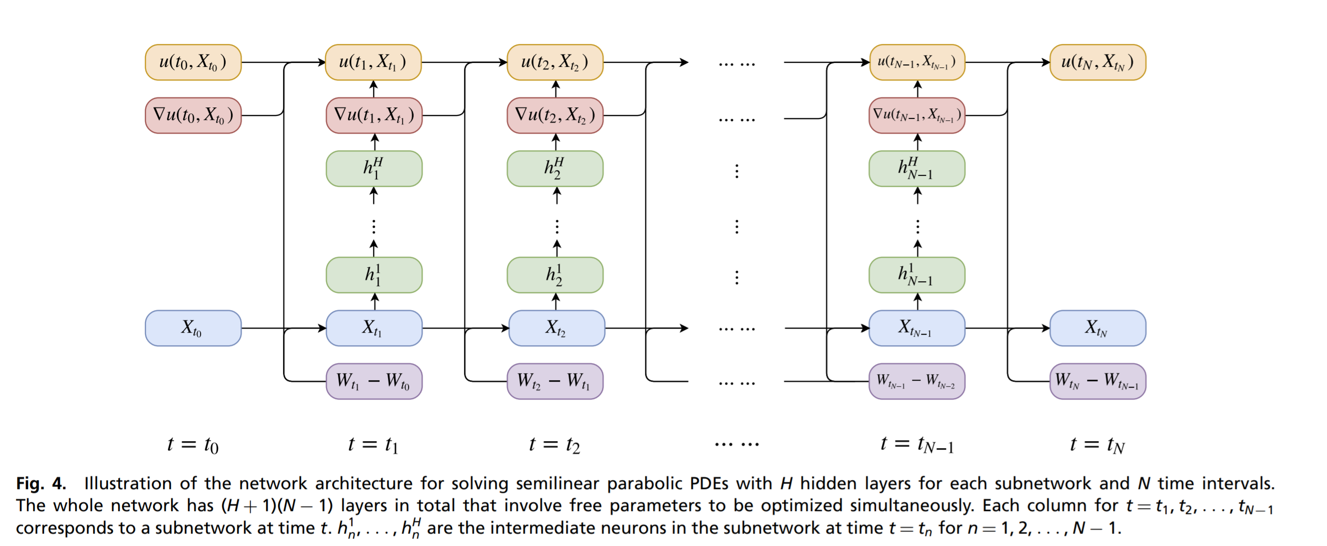
Julia Implementation
A Julia implementation for the deep BSDE method can be found at NeuralPDE.jl. The examples considered below are part of the standard test suite.
Financial Applications of Deep BSDEs: Nonlinear Black-Scholes
Now let's look at a few applications which have PDEs that are solved by this method. One set of problems that are solved, given our setup, are Black-Scholes types of equations. Unlike a lot of previous literature, this works for a wide class of nonlinear extensions to Black-Scholes with large portfolios. Here, the dimension of the PDE for $V(t,x)$ is the dimension of $x$, where the dimension is the number of stocks in the portfolio that we want to consider. If we want to track 1000 stocks, this means our PDE is 1000 dimensional! Traditional PDE solvers would need around $N^{1000}$ points evolving over time in order to arrive at the solution, which is completely impractical.
One example of a nonlinear Black-Scholes equation in this form is the Black-Scholes equation with default risk. Here we are adding to the standard model the idea that the companies that we are buying stocks for can default, and thus our valuation has to take into account this default probability as the option will thus become value-less. The PDE that is arrived at is:
\[ \frac{\partial u}{\partial t}(t,x) + \bar{\mu}\cdot \nabla u(t, x) + \frac{\bar{\sigma}^{2}}{2} \sum_{i=1}^{d} \left |x_{i} \right |^{2} \frac{\partial^2 u}{\partial {x_{i}}^2}(t,x) \\ - (1 -\delta )Q(u(t,x))u(t,x) - Ru(t,x) = 0 \]
with terminating condition $g(x) = \min_{i} x_i$ for $x = (x_{1}, . . . , x_{100}) \in R^{100}$, where $\delta \in [0, 1)$, $R$ is the interest rate of the risk-free asset, and Q is a piecewise linear function of the current value with three regions $(v^{h} < v ^{l}, \gamma^{h} > \gamma^{l})$,
\[ \begin{align} Q(y) &= \mathbb{1}_{(-\infty,\upsilon^{h})}(y)\gamma ^{h} + \mathbb{1}_{[\upsilon^{l},\infty)}(y)\gamma ^{l} \\ &+ \mathbb{1}_{[\upsilon^{h},\upsilon^{l}]}(y) \left[ \frac{(\gamma ^{h} - \gamma ^{l})}{(\upsilon ^{h}- \upsilon ^{l})} (y - \upsilon ^{h}) + \gamma ^{h} \right ]. \end{align} \]
This PDE can be cast into the form of the deep BSDE method by setting:
\[ \begin{align} \mu &= \overline{\mu} X_{t} \\ \sigma &= \overline{\sigma} \text{diag}(X_{t}) \\ f &= -(1 -\delta )Q(u(t,x))u(t,x) - R u(t,x) \end{align} \]
The Julia code for this exact problem in 100 dimensions can be found here
Stochastic Optimal Control as a Deep BSDE Application
Another type of problem that fits into this terminal PDE form is the stochastic optimal control problem. The problem is a generalized context to what motivated us before. In this case, there are a set of agents which undergo some known stochastic model. What we want to do is apply some control (push them in some direction) at every single timepoint towards some goal. For example, we have the physics for the dynamics of drone flight, but there's randomness in the wind condition, and so we want to control the engine speeds to move in a certain direction. However, there is a cost associated with controlling, and thus the question is how to best balance the use of controls with the natural stochastic evolution.
It turns out this is in the same form as the Black-Scholes problem. There is a model evolving forwards, and when we get to the end we know how much everything "cost" because we know if the drone got to the right location and how much energy it took. So in the same sense as Black-Scholes, we can know the value at the end and try and propagate it backwards given the current state of the system $x$, to find out $u(0,\zeta)$, i.e. how should we control right now given the current system is in the state $x = \zeta$. It turns out that the solution of $u(t,x)$ where $u(T,x)=g(x)$ and we want to find $u(0,\zeta)$ is given by a partial differential equation which is known as the Hamilton-Jacobi-Bellman equation, which is one of these terminal PDEs that is representable by the deep BSDE method.
Take the classical linear-quadratic Gaussian (LQG) control problem in 100 dimensions
\[ dX_t = 2\sqrt{\lambda} c_t dt + \sqrt{2} dW_t \]
with $t\in [0,T]$, $X_0 = x$, and with a cost function
\[ C(c_t) = \mathbb{E}\left[\int_0^T \Vert c_t \Vert_2^2 dt + g(X_t) \right] \]
where $X_t$ is the state we wish to control, $\lambda$ is the strength of the control, and $c_t$ is the control process. To minimize the control, the Hamilton–Jacobi–Bellman equation:
\[ \frac{\partial u}{\partial t}(t,x) + \Delta u(t,x) - \lambda \Vert \nabla u(t,x) \Vert_2^2 = 0 \]
has a solution $u(t,x)$ which at $t=0$ represents the optimal cost of starting from $x$.
This PDE can be rewritten into the canonical form of the deep BSDE method by setting:
\[ \begin{align} \mu &= 0, \\ \sigma &= \overline{\sigma} I, \\ f &= -\alpha \left \| \sigma^T(s,X_s)\nabla u(s,X_s)) \right \|_2^{2}, \end{align} \]
where $\overline{\sigma} = \sqrt{2}$, T = 1 and $X_0 = (0,. . . , 0) \in R^{100}$.
The Julia code for solving this exact problem in 100 dimensions can be found here
Connections of Reservoir Computing to Scientific Machine Learning
Reservoir computing techniques are an alternative to the "full" neural network techniques we have previously discussed. However, the process of training neural networks has a few caveats which can cause difficulties in real systems:
The tangent space diverges exponentially fast when the system is chaotic, meaning that results of both forward and reverse automatic differentiation techniques (and the related adjoints) are divergent on these kinds of systems.
It is hard for neural networks to represent stiff systems. There are many reasons for this, one being that neural networks tend to drop high frequency behavior.
There are ways being investigated to alleviate these issues. For example, shadow adjoints can give a non-divergent average sense of a derivative on ergodic chaotic systems, but is significantly more expensive than the traditional adjoint.
To get around these caveats, some research teams have investigated alternatives which do not require gradient-based optimization. The clear frontrunner in this field is a type of architecture called echo state networks. A simplified formulation of an echo state network essentially fixes a neural network that defines a reservoir, i.e.
\[ x_{n+1} = \sigma(W x_n + W_{fb} y_n) \]
\[ y_n = g(W_{out} x_n) \]
where $W$ and $W_{fb}$ are fixed random matrices that are chosen before the training process, $x_n$ is called the reservoir state, and $y_n$ is the output state for the observables. The idea is to find a projection $W_{out}$ from the high dimensional random reservoir $x$ to model the timeseries by $y$. If the reservoir is a big enough and nonlinear enough random system, there should in theory exist a projection from that random system that matches any potential timeseries. Indeed, one can prove that echo state networks are universal adaptive filters under certain conditions.
If $g$ is invertible (and in many cases $g$ is taken to be the identity), then one can directly apply the inversion of $g$ to the data. This turns the training of $W_{out}$, the only non-fixed portion, into a standard least squares regression between the reservoir and the observation series. This is then solved by classical means like SVD factorizations which can be stable in ill-conditioned cases.
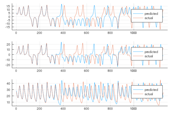
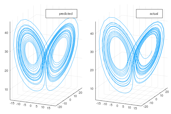
Echo state networks have been shown to accurately reproduce chaotic attractors which are shown to be hard to train RNNs against. A demonstration via ReservoirComputing.jl clearly highlights this prediction ability:
However, this methodology still is not tailored to the continuous nature of dynamical systems found in scientific computing. Recent work has extended this methodolgy to allow for a continuous reservoir, i.e. a continuous-time echo state network. It is shown that using the adaptive points of a stiff ODE integrator gives a non-uniform sampling in time that makes it easier to learn stiff equations from less training points, and demonstrates the ability to learn equations where standard physics-informed neural network (PINN) training techniques fail.
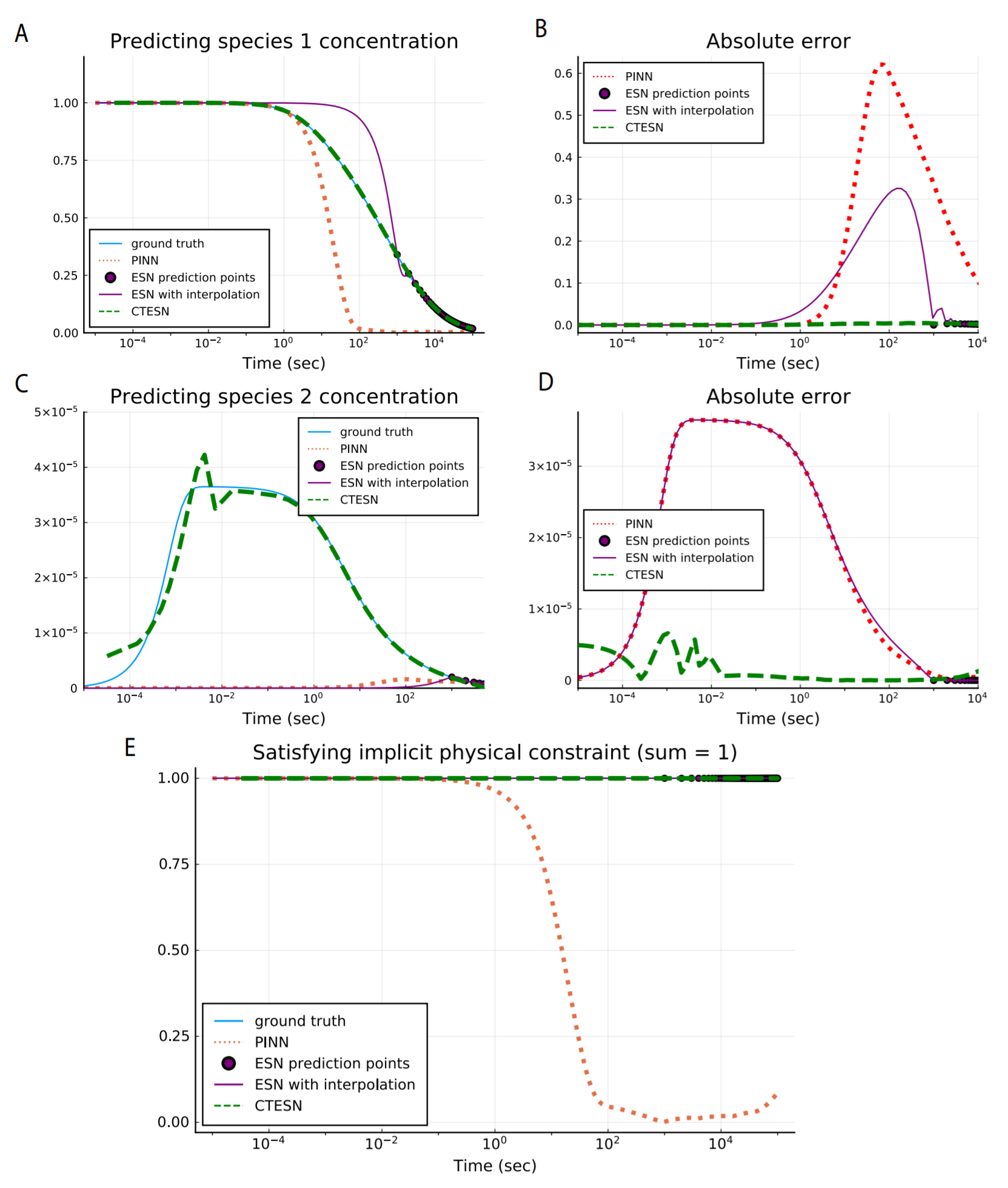
This area of research is still far less developed than PINNs and neural differential equations but shows promise to more easily learn highly stiff and chaotic systems which are seemingly out of reach for these other methods.
Automated Equation Discovery: Outputting LaTeX for Dynamical Systems from Data
The SINDy algorithm enables data-driven discovery of governing equations from data. It leverages the fact that most physical systems have only a few relevant terms that define the dynamics, making the governing equations sparse in a high-dimensional nonlinear function space. Given a set of observations
\[ \begin{array}{c} \mathbf{X}=\left[\begin{array}{c} \mathbf{x}^{T}\left(t_{1}\right) \\ \mathbf{x}^{T}\left(t_{2}\right) \\ \vdots \\ \mathbf{x}^{T}\left(t_{m}\right) \end{array}\right]=\left[\begin{array}{cccc} x_{1}\left(t_{1}\right) & x_{2}\left(t_{1}\right) & \cdots & x_{n}\left(t_{1}\right) \\ x_{1}\left(t_{2}\right) & x_{2}\left(t_{2}\right) & \cdots & x_{n}\left(t_{2}\right) \\ \vdots & \vdots & \ddots & \vdots \\ x_{1}\left(t_{m}\right) & x_{2}\left(t_{m}\right) & \cdots & x_{n}\left(t_{m}\right) \end{array}\right] \\ \end{array} \]
and a set of derivative observations
\[ \begin{array}{c} \dot{\mathbf{X}}=\left[\begin{array}{c} \dot{\mathbf{x}}^{T}\left(t_{1}\right) \\ \dot{\mathbf{x}}^{T}\left(t_{2}\right) \\ \vdots \\ \dot{\mathbf{x}}^{T}\left(t_{m}\right) \end{array}\right]=\left[\begin{array}{cccc} \dot{x}_{1}\left(t_{1}\right) & \dot{x}_{2}\left(t_{1}\right) & \cdots & \dot{x}_{n}\left(t_{1}\right) \\ \dot{x}_{1}\left(t_{2}\right) & \dot{x}_{2}\left(t_{2}\right) & \cdots & \dot{x}_{n}\left(t_{2}\right) \\ \vdots & \vdots & \ddots & \vdots \\ \dot{x}_{1}\left(t_{m}\right) & \dot{x}_{2}\left(t_{m}\right) & \cdots & \dot{x}_{n}\left(t_{m}\right) \end{array}\right] \end{array} \]
we can evaluate the observations in a basis $\Theta(X)$:
\[ \Theta(\mathbf{X})=\left[\begin{array}{llllllll} 1 & \mathbf{X} & \mathbf{X}^{P_{2}} & \mathbf{X}^{P_{3}} & \cdots & \sin (\mathbf{X}) & \cos (\mathbf{X}) & \cdots \end{array}\right] \]
where $X^{P_i}$ stands for all $P_i$th order polynomial terms. For example,
\[ \mathbf{X}^{P_{2}}=\left[\begin{array}{cccccc} x_{1}^{2}\left(t_{1}\right) & x_{1}\left(t_{1}\right) x_{2}\left(t_{1}\right) & \cdots & x_{2}^{2}\left(t_{1}\right) & \cdots & x_{n}^{2}\left(t_{1}\right) \\ x_{1}^{2}\left(t_{2}\right) & x_{1}\left(t_{2}\right) x_{2}\left(t_{2}\right) & \cdots & x_{2}^{2}\left(t_{2}\right) & \cdots & x_{n}^{2}\left(t_{2}\right) \\ \vdots & \vdots & \ddots & \vdots & \ddots & \vdots \\ x_{1}^{2}\left(t_{m}\right) & x_{1}\left(t_{m}\right) x_{2}\left(t_{m}\right) & \cdots & x_{2}^{2}\left(t_{m}\right) & \cdots & x_{n}^{2}\left(t_{m}\right) \end{array}\right] \]
Using these matrices, SINDy finds this sparse basis $\mathbf{\Xi}$ over a given candidate library $\mathbf{\Theta}$ by solving the sparse regression problem $\dot{X} =\mathbf{\Theta}\mathbf{\Xi}$ with $L_1$ regularization, i.e. minimizing the objective function $\left\Vert \mathbf{\dot{X}} - \mathbf{\Theta}\mathbf{\Xi} \right\Vert_2 + \lambda \left\Vert \mathbf{\Xi}\right\Vert_1$. This method and other variants of SInDy, along with specialized optimizers for the LASSO $L_1$ optimization problem, have been implemented in packages like DataDrivenDiffEq.jl and pysindy. The result of these methods is LaTeX for the missing dynamical system.
Notice that to use this method, derivative data $\dot{X}$ is required. While in most publications on the subject this information is assumed. To find this, $\dot{X}$ is calculated directly from the time series $X$ by fitting a cubic spline and taking the approximated derivatives at the observation points. However, for this estimation to be stable one needs a fairly dense timeseries for the interpolation. To alleviate this issue, the universal differential equations work estimates terms of partially described models and then uses the neural network as an oracle for the derivative values to learn from subsets of the dynamical system. This allows for the neural network's training to smooth out the derivative estimate between points while incorporating extra scientific information.
Other ways are being investigated for incorporating deep learning into the model discovery process. For example, extensions have been investigated where elements are defined by neural networks representing a basis of the Koopman operator. Additionally, much work is going on in improving the efficiency of the symbolic regression methods themselves, and making the methods implicit and parallel.
Surrogate Acceleration Methods
Another approach for mixing neural networks with differential equations is as a surrogate method. These methods are more mathematically trivial than the previous ideas, but can still achieve interesting results. A full example is explained in this video.
Say we have some function $g(p)$ which depends on a solution to a differential equation $u(t;p)$ and choices of parameters $p$. Computationally how we evaluate this function is we do the following:
Solve the differential equation with parameters $p$
Evaluate $g$ on the numerical solution for $u$
However, this process is computationally expensive since it requires the numerical solution of $u$ for every evaluation. Thus, one can look at this setup and see $g(p)$ itself is a nonlinear function. The idea is to train a neural network to be the function $g(p)$, i.e. directly put in $p$ and return the appropriate value without ever solving the differential equation.
The video highlights an important fact about this method: it can be computationally expensive to train this kind of surrogate since many data points $(p,g(p))$ are required. In fact, many more data points than you might use. However, after training, the surrogate network for $g(p)$ can be a lot faster than the original simulation-based approach. This means that this is a method for accelerating real-time solutions by doing upfront computations. The total compute time will always be more, but in some sense the cost is amortized or shifted to be done before hand, so that the model does not need to be simulated on the fly. This can allow for things like computationally expensive models of drone flight to be used in a real-time controller.
This technique goes a long way back, but some recent examples of this have been shown. For example, there's this paper which "accelerated" the solution of the 3-body problem using a neural network surrogate trained over a few days to get a 1 million times acceleration (after generating many points beforehand of course! In the paper, notice that it took 10 days to generate the training dataset). Additionally, there is this deep learning trebuchet example which showcased that inverse problems, i.e. control or finding parameters, can be completely encapsulated as a $g(p)$ and learned with sufficient data.