The Different Flavors of Parallelism
Chris Rackauckas
September 25th, 2020
Youtube Video Link
Now that you are aware of the basics of parallel computing, let's give a high level overview of the differences between different modes of parallelism.
Lowest Level: SIMD
Recall SIMD, the idea that processors can run multiple commands simultaneously on specially structured data. "Single Instruction Multiple Data". SIMD is parallelism within a single core.
High Level Idea of SIMD
Calculations can occur in parallel in the processor if there is sufficient structure in the computation.
How to do SIMD
The simplest way to do SIMD is simply to make sure that your values are aligned. If they are, then great, LLVM's autovectorizer pass has a good chance of automatic vectorization (in the world of computing, "SIMD" is synonymous with vectorization since it is taking specific values and instead computing on small vectors. That is not to be confused with "vectorization" in the sense of Python/R/MATLAB, which is a programming style which prefers using C-defined primitive functions, like broadcast or matrix multiplication).
You can check for auto-vectorization inside of the LLVM IR by looking for statements like:
%wide.load24 = load <4 x double>, <4 x double> addrspac(13)* %46, align 8
; └
; ┌ @ float.jl:395 within `+'
%47 = fadd <4 x double> %wide.load, %wide.load24
which means that 4 additions are happening simultaneously. The amount of vectorization is heavily dependent on your architecture. The ancient form of SIMD, the SSE(2) instructions, required that your data was aligned. Now there's a bit more leeway, but generally it holds that making your the data you're trying to SIMD over is aligned. Thus there can be major differences in computing using a struct of array format instead of an arrays of structs format. For example:
struct MyComplex
  real::Float64
  imag::Float64
end
arr = [MyComplex(rand(),rand()) for i in 1:100]
100-element Vector{MyComplex}:
 MyComplex(0.34747659865291214, 0.19840029638184054)
 MyComplex(0.8256234273325588, 0.024156565649226636)
 MyComplex(0.6289449315742727, 0.2126560063488352)
 MyComplex(0.8830892542017056, 0.3877715747499726)
 MyComplex(0.02516588330429137, 0.7744466006343095)
 MyComplex(0.6372108737424679, 0.8224823999862052)
 MyComplex(0.21087481812513298, 0.5590703315363701)
 MyComplex(0.21261419853597407, 0.9165601772286993)
 MyComplex(0.22065610631024513, 0.801015134289168)
 MyComplex(0.9895225697316358, 0.12869584824441804)
 ⋮
 MyComplex(0.034821884129790925, 0.3757044479973688)
 MyComplex(0.8306208596445002, 0.5377547763154478)
 MyComplex(0.21189238057457205, 0.4668621553740182)
 MyComplex(0.36701711146425287, 0.3108439744128483)
 MyComplex(0.04956542712834122, 0.1563261979712246)
 MyComplex(0.0503024799176629, 0.6250976663625579)
 MyComplex(0.6775781909720691, 0.8485946386428548)
 MyComplex(0.6986484642620416, 0.8980389038900529)
 MyComplex(0.796904411621678, 0.5017204294402445)
is represented in memory as
[real1,imag1,real2,imag2,...]while the struct of array formats are
struct MyComplexes
  real::Vector{Float64}
  imag::Vector{Float64}
end
arr2 = MyComplexes(rand(100),rand(100))
MyComplexes([0.7539756667194848, 0.20455149361509817, 0.96770587729343, 0.2
6491948886353567, 0.28671038901712975, 0.47832023299044035, 0.3146400367888
62, 0.8689061404510314, 0.8371060390408374, 0.7746621135875877  …  0.527978
6671954683, 0.19821939560362278, 0.36237221339519643, 0.8620577651458297, 0
.6058560069690415, 0.41626321585554305, 0.3067396498717959, 0.4587321869029
759, 0.9889932371944905, 0.04954520213683067], [0.9202055282502578, 0.49627
5947326719, 0.3950111630972739, 0.9862492688947864, 0.3703209744831629, 0.7
253227319751944, 0.8784957341805517, 0.9303480388087012, 0.5727206525583906
, 0.25751476686393215  …  0.263407004452754, 0.34654878085128626, 0.2650742
616611541, 0.8852099069175132, 0.01261919256406041, 0.8378126744225836, 0.2
8532342961264845, 0.8069850589300858, 0.7043141109486648, 0.899226007012973
2])
Now let's check what happens when we perform a reduction:
using InteractiveUtils
Base.:+(x::MyComplex,y::MyComplex) = MyComplex(x.real+y.real,x.imag+y.imag)
Base.:/(x::MyComplex,y::Int) = MyComplex(x.real/y,x.imag/y)
average(x::Vector{MyComplex}) = sum(x)/length(x)
@code_llvm average(arr)
; Function Signature: average(Array{Main.MyComplex, 1})
;  @ /home/runner/work/SciMLBook/SciMLBook/_weave/lecture06/styles_of_paral
lelism.jmd:5 within `average`
define void @julia_average_83180(ptr noalias nocapture noundef nonnull sret
([2 x double]) align 8 dereferenceable(16) %sret_return, ptr noundef nonnul
l align 8 dereferenceable(24) %"x::Array") #0 {
top:
  %jlcallframe1 = alloca [4 x ptr], align 8
  %sret_box = alloca [2 x i64], align 8
; ┌ @ reducedim.jl:979 within `sum`
; │┌ @ reducedim.jl:979 within `#sum#735`
; ││┌ @ reducedim.jl:983 within `_sum`
; │││┌ @ reducedim.jl:983 within `#_sum#737`
; ││││┌ @ reducedim.jl:984 within `_sum`
; │││││┌ @ reducedim.jl:984 within `#_sum#738`
; ││││││┌ @ reducedim.jl:326 within `mapreduce`
; │││││││┌ @ reducedim.jl:326 within `#mapreduce#728`
; ││││││││┌ @ reducedim.jl:334 within `_mapreduce_dim`
; │││││││││┌ @ reduce.jl:418 within `_mapreduce`
; ││││││││││┌ @ indices.jl:536 within `LinearIndices`
; │││││││││││┌ @ abstractarray.jl:98 within `axes`
; ││││││││││││┌ @ array.jl:194 within `size`
               %"x::Array.size_ptr" = getelementptr inbounds i8, ptr %"x::A
rray", i64 16
               %"x::Array.size.0.copyload" = load i64, ptr %"x::Array.size_
ptr", align 8
; ││││││││││└└└
; ││││││││││ @ reduce.jl:420 within `_mapreduce`
            switch i64 %"x::Array.size.0.copyload", label %L29 [
    i64 0, label %L6
    i64 1, label %guard_pass61
  ]

L6:                                               ; preds = %top
; ││││││││││ @ reduce.jl:421 within `_mapreduce`
            store ptr @"jl_global#83185.jit", ptr %jlcallframe1, align 8
            %0 = getelementptr inbounds ptr, ptr %jlcallframe1, i64 1
            store ptr @"jl_global#83186.jit", ptr %0, align 8
            %1 = getelementptr inbounds ptr, ptr %jlcallframe1, i64 2
            store ptr %"x::Array", ptr %1, align 8
            %2 = getelementptr inbounds ptr, ptr %jlcallframe1, i64 3
            store ptr @"jl_global#83187.jit", ptr %2, align 8
            %3 = call nonnull ptr @j1_mapreduce_empty_iter_83183(ptr nonnul
l @"jl_global#83184.jit", ptr nonnull %jlcallframe1, i32 4)
            call void @llvm.trap()
            unreachable

L29:                                              ; preds = %top
; ││││││││││ @ reduce.jl:425 within `_mapreduce`
; ││││││││││┌ @ int.jl:83 within `<`
             %4 = icmp sgt i64 %"x::Array.size.0.copyload", 15
; ││││││││││└
            br i1 %4, label %guard_pass71, label %guard_exit77

L108.loopexit.unr-lcssa:                          ; preds = %guard_exit82,
%guard_exit82.preheader
            %.lcssa.ph = phi <2 x double> [ undef, %guard_exit82.preheader
], [ %39, %guard_exit82 ]
            %value_phi38106.unr = phi i64 [ 2, %guard_exit82.preheader ], [
 %37, %guard_exit82 ]
            %.unr = phi <2 x double> [ %18, %guard_exit82.preheader ], [ %3
9, %guard_exit82 ]
; ││││││││││ @ reduce.jl:430 within `_mapreduce`
            %lcmp.mod.not = icmp eq i64 %xtraiter, 0
            br i1 %lcmp.mod.not, label %L108, label %guard_exit82.epil

guard_exit82.epil:                                ; preds = %guard_exit82.e
pil, %L108.loopexit.unr-lcssa
            %value_phi38106.epil = phi i64 [ %6, %guard_exit82.epil ], [ %v
alue_phi38106.unr, %L108.loopexit.unr-lcssa ]
            %5 = phi <2 x double> [ %8, %guard_exit82.epil ], [ %.unr, %L10
8.loopexit.unr-lcssa ]
            %epil.iter = phi i64 [ %epil.iter.next, %guard_exit82.epil ], [
 0, %L108.loopexit.unr-lcssa ]
; ││││││││││ @ reduce.jl:431 within `_mapreduce`
; ││││││││││┌ @ int.jl:87 within `+`
             %6 = add nuw nsw i64 %value_phi38106.epil, 1
; ││││││││││└
; ││││││││││┌ @ essentials.jl:920 within `getindex`
             %memoryref_byteoffset.epil = shl i64 %value_phi38106.epil, 4
             %memoryref_data50.epil = getelementptr inbounds i8, ptr %memor
yref_data14, i64 %memoryref_byteoffset.epil
             %7 = load <2 x double>, ptr %memoryref_data50.epil, align 8
; ││││││││││└
; ││││││││││ @ reduce.jl:432 within `_mapreduce`
; ││││││││││┌ @ reduce.jl:16 within `add_sum`
; │││││││││││┌ @ /home/runner/work/SciMLBook/SciMLBook/_weave/lecture06/sty
les_of_parallelism.jmd:3 within `+` @ float.jl:495
              %8 = fadd <2 x double> %5, %7
; ││││││││││└└
; ││││││││││ @ reduce.jl:430 within `_mapreduce`
            %epil.iter.next = add i64 %epil.iter, 1
            %epil.iter.cmp.not = icmp eq i64 %epil.iter.next, %xtraiter
            br i1 %epil.iter.cmp.not, label %L108, label %guard_exit82.epil

L108:                                             ; preds = %guard_exit77,
%guard_pass71, %guard_pass61, %guard_exit82.epil, %L108.loopexit.unr-lcssa
; └└└└└└└└└└
; ┌ @ essentials.jl:11 within `length`
   %"x::Array.size6.0.copyload" = phi i64 [ %"x::Array.size6.0.copyload.pre
", %guard_pass71 ], [ 1, %guard_pass61 ], [ %"x::Array.size.0.copyload", %g
uard_exit77 ], [ %"x::Array.size.0.copyload", %guard_exit82.epil ], [ %"x::
Array.size.0.copyload", %L108.loopexit.unr-lcssa ]
   %9 = phi <2 x double> [ %15, %guard_pass71 ], [ %14, %guard_pass61 ], [
%18, %guard_exit77 ], [ %.lcssa.ph, %L108.loopexit.unr-lcssa ], [ %8, %guar
d_exit82.epil ]
; └
; ┌ @ /home/runner/work/SciMLBook/SciMLBook/_weave/lecture06/styles_of_para
llelism.jmd:4 within `/` @ promotion.jl:436
; │┌ @ promotion.jl:404 within `promote`
; ││┌ @ promotion.jl:379 within `_promote`
; │││┌ @ number.jl:7 within `convert`
; ││││┌ @ float.jl:245 within `Float64`
       %10 = sitofp i64 %"x::Array.size6.0.copyload" to double
; │└└└└
; │ @ /home/runner/work/SciMLBook/SciMLBook/_weave/lecture06/styles_of_para
llelism.jmd:4 within `/` @ promotion.jl:436 @ float.jl:498
   %11 = insertelement <2 x double> poison, double %10, i64 0
   %12 = shufflevector <2 x double> %11, <2 x double> poison, <2 x i32> zer
oinitializer
   %13 = fdiv <2 x double> %9, %12
; │ @ /home/runner/work/SciMLBook/SciMLBook/_weave/lecture06/styles_of_para
llelism.jmd:4 within `/`
; │┌ @ /home/runner/work/SciMLBook/SciMLBook/_weave/lecture06/styles_of_par
allelism.jmd:3 within `MyComplex`
    store <2 x double> %13, ptr %sret_return, align 8
    ret void

guard_pass61:                                     ; preds = %top
; └└
; ┌ @ reducedim.jl:979 within `sum`
; │┌ @ reducedim.jl:979 within `#sum#735`
; ││┌ @ reducedim.jl:983 within `_sum`
; │││┌ @ reducedim.jl:983 within `#_sum#737`
; ││││┌ @ reducedim.jl:984 within `_sum`
; │││││┌ @ reducedim.jl:984 within `#_sum#738`
; ││││││┌ @ reducedim.jl:326 within `mapreduce`
; │││││││┌ @ reducedim.jl:326 within `#mapreduce#728`
; ││││││││┌ @ reducedim.jl:334 within `_mapreduce_dim`
; │││││││││┌ @ reduce.jl:423 within `_mapreduce`
; ││││││││││┌ @ essentials.jl:920 within `getindex`
             %memoryref_data = load ptr, ptr %"x::Array", align 8
             %14 = load <2 x double>, ptr %memoryref_data, align 8
             br label %L108

guard_pass71:                                     ; preds = %L29
; ││││││││││└
; ││││││││││ @ reduce.jl:436 within `_mapreduce`
; ││││││││││┌ @ reduce.jl:269 within `mapreduce_impl`
             call void @j_mapreduce_impl_83189(ptr noalias nocapture nounde
f nonnull sret([2 x double]) align 8 %sret_box, ptr nonnull %"x::Array", i6
4 signext 1, i64 signext %"x::Array.size.0.copyload", i64 signext 1024)
; └└└└└└└└└└└
  %15 = load <2 x double>, ptr %sret_box, align 8
; ┌ @ essentials.jl:11 within `length`
   %"x::Array.size6.0.copyload.pre" = load i64, ptr %"x::Array.size_ptr", a
lign 8
   br label %L108

guard_exit77:                                     ; preds = %L29
; └
; ┌ @ reducedim.jl:979 within `sum`
; │┌ @ reducedim.jl:979 within `#sum#735`
; ││┌ @ reducedim.jl:983 within `_sum`
; │││┌ @ reducedim.jl:983 within `#_sum#737`
; ││││┌ @ reducedim.jl:984 within `_sum`
; │││││┌ @ reducedim.jl:984 within `#_sum#738`
; ││││││┌ @ reducedim.jl:326 within `mapreduce`
; │││││││┌ @ reducedim.jl:326 within `#mapreduce#728`
; ││││││││┌ @ reducedim.jl:334 within `_mapreduce_dim`
; │││││││││┌ @ reduce.jl:427 within `_mapreduce`
; ││││││││││┌ @ essentials.jl:920 within `getindex`
             %memoryref_data14 = load ptr, ptr %"x::Array", align 8
; ││││││││││└
; ││││││││││ @ reduce.jl:428 within `_mapreduce`
; ││││││││││┌ @ essentials.jl:920 within `getindex`
             %memoryref_data31 = getelementptr inbounds i8, ptr %memoryref_
data14, i64 16
; ││││││││││└
; ││││││││││ @ reduce.jl:427 within `_mapreduce`
; ││││││││││┌ @ essentials.jl:920 within `getindex`
             %16 = load <2 x double>, ptr %memoryref_data14, align 8
; ││││││││││└
; ││││││││││ @ reduce.jl:428 within `_mapreduce`
; ││││││││││┌ @ essentials.jl:920 within `getindex`
             %17 = load <2 x double>, ptr %memoryref_data31, align 8
; ││││││││││└
; ││││││││││ @ reduce.jl:429 within `_mapreduce`
; ││││││││││┌ @ reduce.jl:16 within `add_sum`
; │││││││││││┌ @ /home/runner/work/SciMLBook/SciMLBook/_weave/lecture06/sty
les_of_parallelism.jmd:3 within `+` @ float.jl:495
              %18 = fadd <2 x double> %16, %17
; ││││││││││└└
; ││││││││││ @ reduce.jl:430 within `_mapreduce`
; ││││││││││┌ @ int.jl:83 within `<`
             %.not102103 = icmp sgt i64 %"x::Array.size.0.copyload", 2
; ││││││││││└
            br i1 %.not102103, label %guard_exit82.preheader, label %L108

guard_exit82.preheader:                           ; preds = %guard_exit77
            %19 = add nsw i64 %"x::Array.size.0.copyload", -2
            %20 = add nsw i64 %"x::Array.size.0.copyload", -3
            %xtraiter = and i64 %19, 7
            %21 = icmp ult i64 %20, 7
            br i1 %21, label %L108.loopexit.unr-lcssa, label %guard_exit82.
preheader.new

guard_exit82.preheader.new:                       ; preds = %guard_exit82.p
reheader
            %unroll_iter = and i64 %19, -8
            br label %guard_exit82

guard_exit82:                                     ; preds = %guard_exit82,
%guard_exit82.preheader.new
            %value_phi38106 = phi i64 [ 2, %guard_exit82.preheader.new ], [
 %37, %guard_exit82 ]
            %22 = phi <2 x double> [ %18, %guard_exit82.preheader.new ], [
%39, %guard_exit82 ]
            %niter = phi i64 [ 0, %guard_exit82.preheader.new ], [ %niter.n
ext.7, %guard_exit82 ]
; ││││││││││ @ reduce.jl:431 within `_mapreduce`
; ││││││││││┌ @ essentials.jl:920 within `getindex`
             %memoryref_byteoffset = shl i64 %value_phi38106, 4
             %memoryref_data50 = getelementptr i8, ptr %memoryref_data14, i
64 %memoryref_byteoffset
             %23 = load <2 x double>, ptr %memoryref_data50, align 8
; ││││││││││└
; ││││││││││ @ reduce.jl:432 within `_mapreduce`
; ││││││││││┌ @ reduce.jl:16 within `add_sum`
; │││││││││││┌ @ /home/runner/work/SciMLBook/SciMLBook/_weave/lecture06/sty
les_of_parallelism.jmd:3 within `+` @ float.jl:495
              %24 = fadd <2 x double> %22, %23
; ││││││││││└└
; ││││││││││ @ reduce.jl:431 within `_mapreduce`
; ││││││││││┌ @ essentials.jl:920 within `getindex`
             %memoryref_byteoffset.1 = or disjoint i64 %memoryref_byteoffse
t, 16
             %memoryref_data50.1 = getelementptr inbounds i8, ptr %memoryre
f_data14, i64 %memoryref_byteoffset.1
             %25 = load <2 x double>, ptr %memoryref_data50.1, align 8
; ││││││││││└
; ││││││││││ @ reduce.jl:432 within `_mapreduce`
; ││││││││││┌ @ reduce.jl:16 within `add_sum`
; │││││││││││┌ @ /home/runner/work/SciMLBook/SciMLBook/_weave/lecture06/sty
les_of_parallelism.jmd:3 within `+` @ float.jl:495
              %26 = fadd <2 x double> %24, %25
; ││││││││││└└
; ││││││││││ @ reduce.jl:431 within `_mapreduce`
; ││││││││││┌ @ essentials.jl:920 within `getindex`
             %memoryref_data50.2 = getelementptr i8, ptr %memoryref_data50,
 i64 32
             %27 = load <2 x double>, ptr %memoryref_data50.2, align 8
; ││││││││││└
; ││││││││││ @ reduce.jl:432 within `_mapreduce`
; ││││││││││┌ @ reduce.jl:16 within `add_sum`
; │││││││││││┌ @ /home/runner/work/SciMLBook/SciMLBook/_weave/lecture06/sty
les_of_parallelism.jmd:3 within `+` @ float.jl:495
              %28 = fadd <2 x double> %26, %27
; ││││││││││└└
; ││││││││││ @ reduce.jl:431 within `_mapreduce`
; ││││││││││┌ @ essentials.jl:920 within `getindex`
             %memoryref_data50.3 = getelementptr i8, ptr %memoryref_data50,
 i64 48
             %29 = load <2 x double>, ptr %memoryref_data50.3, align 8
; ││││││││││└
; ││││││││││ @ reduce.jl:432 within `_mapreduce`
; ││││││││││┌ @ reduce.jl:16 within `add_sum`
; │││││││││││┌ @ /home/runner/work/SciMLBook/SciMLBook/_weave/lecture06/sty
les_of_parallelism.jmd:3 within `+` @ float.jl:495
              %30 = fadd <2 x double> %28, %29
; ││││││││││└└
; ││││││││││ @ reduce.jl:431 within `_mapreduce`
; ││││││││││┌ @ essentials.jl:920 within `getindex`
             %memoryref_data50.4 = getelementptr i8, ptr %memoryref_data50,
 i64 64
             %31 = load <2 x double>, ptr %memoryref_data50.4, align 8
; ││││││││││└
; ││││││││││ @ reduce.jl:432 within `_mapreduce`
; ││││││││││┌ @ reduce.jl:16 within `add_sum`
; │││││││││││┌ @ /home/runner/work/SciMLBook/SciMLBook/_weave/lecture06/sty
les_of_parallelism.jmd:3 within `+` @ float.jl:495
              %32 = fadd <2 x double> %30, %31
; ││││││││││└└
; ││││││││││ @ reduce.jl:431 within `_mapreduce`
; ││││││││││┌ @ essentials.jl:920 within `getindex`
             %memoryref_data50.5 = getelementptr i8, ptr %memoryref_data50,
 i64 80
             %33 = load <2 x double>, ptr %memoryref_data50.5, align 8
; ││││││││││└
; ││││││││││ @ reduce.jl:432 within `_mapreduce`
; ││││││││││┌ @ reduce.jl:16 within `add_sum`
; │││││││││││┌ @ /home/runner/work/SciMLBook/SciMLBook/_weave/lecture06/sty
les_of_parallelism.jmd:3 within `+` @ float.jl:495
              %34 = fadd <2 x double> %32, %33
; ││││││││││└└
; ││││││││││ @ reduce.jl:431 within `_mapreduce`
; ││││││││││┌ @ essentials.jl:920 within `getindex`
             %memoryref_data50.6 = getelementptr i8, ptr %memoryref_data50,
 i64 96
             %35 = load <2 x double>, ptr %memoryref_data50.6, align 8
; ││││││││││└
; ││││││││││ @ reduce.jl:432 within `_mapreduce`
; ││││││││││┌ @ reduce.jl:16 within `add_sum`
; │││││││││││┌ @ /home/runner/work/SciMLBook/SciMLBook/_weave/lecture06/sty
les_of_parallelism.jmd:3 within `+` @ float.jl:495
              %36 = fadd <2 x double> %34, %35
; ││││││││││└└
; ││││││││││ @ reduce.jl:431 within `_mapreduce`
; ││││││││││┌ @ int.jl:87 within `+`
             %37 = add nuw nsw i64 %value_phi38106, 8
; ││││││││││└
; ││││││││││┌ @ essentials.jl:920 within `getindex`
             %memoryref_data50.7 = getelementptr i8, ptr %memoryref_data50,
 i64 112
             %38 = load <2 x double>, ptr %memoryref_data50.7, align 8
; ││││││││││└
; ││││││││││ @ reduce.jl:432 within `_mapreduce`
; ││││││││││┌ @ reduce.jl:16 within `add_sum`
; │││││││││││┌ @ /home/runner/work/SciMLBook/SciMLBook/_weave/lecture06/sty
les_of_parallelism.jmd:3 within `+` @ float.jl:495
              %39 = fadd <2 x double> %36, %38
; ││││││││││└└
; ││││││││││ @ reduce.jl:430 within `_mapreduce`
            %niter.next.7 = add i64 %niter, 8
            %niter.ncmp.7 = icmp eq i64 %niter.next.7, %unroll_iter
            br i1 %niter.ncmp.7, label %L108.loopexit.unr-lcssa, label %gua
rd_exit82
; └└└└└└└└└└
}
What this is doing is creating small little vectors and then parallelizing the operations of those vectors by calling specific vector-parallel instructions. Keep this in mind.
Explicit SIMD
The following was all a form of loop-level parallelism known as loop vectorization. It's simply easier for compilers to reason at the array level, prove iterates are independent, and automatically generate SIMD code from that. This is not necessary, and compilers can produce SIMD code from non-looping code through a process known as SLP supervectorization, but the results are far from optimal and the compiler requires a lot of time to do this calculation, meaning that it's usually not a pass used by default.
If you want to pack the vectors yourself, then primitives for doing so from within Julia are available in SIMD.jl. This is for "real" performance warriors. This looks like for example:
using SIMD
v = Vec{4,Float64}((1,2,3,4))
@show v+v # basic arithmetic is supported
@show sum(v) # basic reductions are supported
v + v = <4 x Float64>[2.0, 4.0, 6.0, 8.0]
sum(v) = 10.0
10.0
Using this you can pull apart code and force the usage of SIMD vectors. One library which makes great use of this is LoopVectorization.jl. However, one word of "caution":
Most performance optimization is not trying to do something really good for performance. Most performance optimization is trying to not do something that is actively bad for performance.
Summary of SIMD
Communication in SIMD is due to locality: if things are local the processor can automatically setup the operations.
There's no real worry about "getting it wrong": you cannot overwrite pieces from different parts of the arithmetic unit, and if SIMD is unsafe then it just won't auto-vectorize.
Suitable for operations measured in ns.
Next Level Up: Multithreading
Last time we briefly went over multithreading and described how every process has multiple threads which share a single heap, and when multiple threads are executed simultaneously we have multithreaded parallelism. Note that you can have multiple threads which aren't executed simultaneously, like in the case of I/O operations, and this is an example of concurrency without parallelism and is commonly referred to as green threads.

Last time we described a simple multithreaded program and noticed that multithreading has an overhead cost of around 50ns-100ns. This is due to the construction of the new stack (among other things) each time a new computational thread is spun up. This means that, unlike SIMD, some thought needs to be put in as to when to perform multithreading: it's not always a good idea. It needs to be high enough on the cost for this to be counter-balanced.
One abstraction that was glossed over was the memory access style. Before, we were considering a single heap, or an UMA style:

However, this is the case for all shared memory devices. For example, compute nodes on the HPC tend to be "dual Xeon" or "quad Xeon", where each Xeon processor is itself a multicore processor. But each processor on its own accesses its own local caches, and thus one has to be aware that this is setup in a NUMA (non-uniform memory access) manner:

where there is a cache that is closer to the processor and a cache that is further away. Care should be taken in this to localize the computation per thread, otherwise a cost associated with the memory sharing will be hit (but all sharing will still be automatic).
In this sense, interthread communication is naturally done through the heap: if you want other threads to be able to touch a value, then you can simply place it on the heap and then it'll be available. We saw this last time by how overlapping computations can re-use the same heap-based caches, meaning that care needs to be taken with how one writes into a dynamically-allocated array.
A simple example that demonstrates this is. First, let's make sure we have multithreading enabled:
using Base.Threads
Threads.nthreads() # should not be 1
4
using BenchmarkTools
acc = 0
@threads for i in 1:10_000
    global acc
    acc += 1
end
acc
2886
The reason for this behavior is that there is a difference between the reading and the writing step to an array. Here, values are being read while other threads are writing, meaning that they see a lower value than when they are attempting to write into it. The result is that the total summation is lower than the true value because of this clashing. We can prevent this by only allowing one thread to utilize the heap-allocated variable at a time. One abstraction for doing this is atomics:
acc = Atomic{Int64}(0)
@threads for i in 1:10_000
    atomic_add!(acc, 1)
end
acc
Atomic{Int64}(10000)
When an atomic add is being done, all other threads wishing to do the same computation are blocked. This of course can have a massive effect on performance since atomic computations are not parallel.
Julia also exposes a lower level of heap control in threading using locks
const acc_lock = Ref{Int64}(0)
const splock = SpinLock()
function f1()
    @threads for i in 1:10_000
        lock(splock)
        acc_lock[] += 1
        unlock(splock)
    end
end
const rsplock = ReentrantLock()
function f2()
    @threads for i in 1:10_000
        lock(rsplock)
        acc_lock[] += 1
        unlock(rsplock)
    end
end
acc2 = Atomic{Int64}(0)
function g()
  @threads for i in 1:10_000
      atomic_add!(acc2, 1)
  end
end
const acc_s = Ref{Int64}(0)
function h()
  global acc_s
  for i in 1:10_000
      acc_s[] += 1
  end
end
@btime f1()
120.897 μs (22 allocations: 1.47 KiB)
SpinLock is non-reentrant, i.e. it will block itself if a thread that calls a lock does another lock. Therefore it has to be used with caution (every lock goes with one unlock), but it's fast. ReentrantLock alleviates those concerns, but trades off a bit of performance:
@btime f2()
133.971 μs (22 allocations: 1.47 KiB)
But if you can use atomics, they will be faster:
@btime g()
104.836 μs (22 allocations: 1.47 KiB)
and if your computation is actually serial, then use serial code:
@btime h()
3.085 ns (0 allocations: 0 bytes)
Why is this so fast? Check the code:
@code_llvm h()
; Function Signature: h()
;  @ /home/runner/work/SciMLBook/SciMLBook/_weave/lecture06/styles_of_paral
lelism.jmd:26 within `h`
define void @julia_h_87503() #0 {
top:
  %"jl_global#87505.jit.promoted" = load i64, ptr @"jl_global#87505.jit", a
lign 8
  %0 = add i64 %"jl_global#87505.jit.promoted", 10000
;  @ /home/runner/work/SciMLBook/SciMLBook/_weave/lecture06/styles_of_paral
lelism.jmd:29 within `h`
  store i64 %0, ptr @"jl_global#87505.jit", align 8
;  @ /home/runner/work/SciMLBook/SciMLBook/_weave/lecture06/styles_of_paral
lelism.jmd:30 within `h`
  ret void
}
It just knows to add 10000. So to get a proper timing let's make the size mutable:
const len = Ref{Int}(10_000)
function h2()
  global acc_s
  global len
  for i in 1:len[]
      acc_s[] += 1
  end
end
@btime h2()
3.095 ns (0 allocations: 0 bytes)
@code_llvm h2()
; Function Signature: h2()
;  @ /home/runner/work/SciMLBook/SciMLBook/_weave/lecture06/styles_of_paral
lelism.jmd:3 within `h2`
define void @julia_h2_87521() #0 {
top:
;  @ /home/runner/work/SciMLBook/SciMLBook/_weave/lecture06/styles_of_paral
lelism.jmd:6 within `h2`
; ┌ @ refvalue.jl:59 within `getindex`
; │┌ @ Base_compiler.jl:54 within `getproperty`
    %.x = load i64, ptr @"jl_global#87523.jit", align 8
; └└
; ┌ @ range.jl:917 within `iterate`
; │┌ @ range.jl:688 within `isempty`
; ││┌ @ operators.jl:425 within `>`
; │││┌ @ int.jl:83 within `<`
      %0 = icmp slt i64 %.x, 1
; └└└└
  br i1 %0, label %L31, label %L17.preheader

L17.preheader:                                    ; preds = %top
  %"jl_global#87524.jit.promoted" = load i64, ptr @"jl_global#87524.jit", a
lign 8
;  @ /home/runner/work/SciMLBook/SciMLBook/_weave/lecture06/styles_of_paral
lelism.jmd:8 within `h2`
  %1 = add i64 %"jl_global#87524.jit.promoted", %.x
;  @ /home/runner/work/SciMLBook/SciMLBook/_weave/lecture06/styles_of_paral
lelism.jmd:7 within `h2`
  store i64 %1, ptr @"jl_global#87524.jit", align 8
;  @ /home/runner/work/SciMLBook/SciMLBook/_weave/lecture06/styles_of_paral
lelism.jmd:8 within `h2`
  br label %L31

L31:                                              ; preds = %L17.preheader,
 %top
  ret void
}
It's still optimizing it!
non_const_len = 10000
function h3()
  global acc_s
  global non_const_len
  len2::Int = non_const_len
  for i in 1:len2
      acc_s[] += 1
  end
end
@btime h3()
12.636 ns (0 allocations: 0 bytes)
Note that what is shown here is a type-declaration. a::T = ... forces a to be of type T throughout the whole function. By giving the compiler this information, I am able to use the non-constant global in a type-stable manner.
One last thing to note about multithreaded computations, and parallel computations, is that one cannot assume that the parallelized computation is computed in any given order. For example, the following will has a quasi-random ordering:
const a2 = zeros(nthreads()*10)
const acc_lock2 = Ref{Int64}(0)
const splock2 = SpinLock()
function f_order()
    @threads for i in 1:length(a2)
        lock(splock2)
        acc_lock2[] += 1
        a2[i] = acc_lock2[]
        unlock(splock2)
    end
end
f_order()
a2
40-element Vector{Float64}:
 12.0
 13.0
 14.0
 15.0
 16.0
 17.0
 18.0
 19.0
 20.0
 21.0
  ⋮
 22.0
 23.0
 24.0
 25.0
 26.0
 27.0
 28.0
 29.0
 30.0
Note that here we can see that Julia 1.5 is dividing up the work into groups of 10 for each thread, and then one thread dominates the computation at a time, but which thread dominates is random.
The Dining Philosophers Problem
A classic tale in parallel computing is the dining philosophers problem. In this case, there are N philosophers at a table who all want to eat at the same time, following all of the same rules. Each philosopher must alternatively think and then eat. They need both their left and right fork to start eating, but cannot start eating until they have both forks. The problem is how to setup a concurrent algorithm that will not cause any philosophers to starve.
The difficulty is a situation known as deadlock. For example, if each philosopher was told to grab the right fork when it's available, and then the left fork, and put down the fork after eating, then they will all grab the right fork and none will ever eat because they will all be waiting on the left fork. This is analogous to two blocked computations which are waiting on the other to finish. Thus, when using blocking structures, one needs to be careful about deadlock!
Two Programming Models: Loop-Level Parallelism and Task-Based Parallelism
As described in the previous lecture, one can also use Threads.@spawn to do multithreading in Julia v1.3+. The same factors all apply: how to do locks and Mutex etc. This is a case of a parallelism construct having two alternative programming models. Threads.@spawn represents task-based parallelism, while Threads.@threads represents Loop-Level Parallelism or a parallel iterator model. Loop-based parallelization models are very high level and, assuming every iteration is independent, almost requires no code change. Task-based parallelism is a more expressive parallelism model, but usually requires modifying the code to be explicitly written as a set of parallelizable tasks. Note that in the case of Julia, Threads.@threads is implemented using Threads.@spawn's model.
Summary of Multithreading
Communication in multithreading is done on the heap. Locks and atomics allow for a form of safe message passing.
50ns-100ns of overhead. Suitable for 1μs calculations.
Be careful of ordering and heap-allocated values.
GPU Computing
GPUs are not fast. In fact, the problem with GPUs is that each processor is slow. However, GPUs have a lot of cores... like thousands.
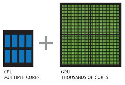
An RTX2080, a standard "gaming" GPU (not even the ones in the cluster), has 2944 cores. However, not only are GPUs slow, but they also need to be programmed in a style that is SPMD, which stands for Single Program Multiple Data. This means that every single thread must be running the same program but on different pieces of data. Exactly the same program. If you have
if a > 1
  # Do something
else
  # Do something else
end
where some of the data goes on one branch and other data goes on the other branch, every single thread will run both branches (performing "fake" computations while on the other branch). This means that GPU tasks should be "very parallel" with as few conditionals as possible.
GPU Memory
GPUs themselves are shared memory devices, meaning they have a heap that is shared amongst all threads. However, GPUs are heavily in the NUMA camp, where different blocks of the GPU have much faster access to certain parts of the memory. Additionally, this heap is disconnected from the standard processor, so data must be passed to the GPU and data must be returned.
GPU memory size is relatively small compared to CPUs. Example: the RTX2080Ti has 8GB of RAM. Thus one needs to be doing computations that are memory compact (such as matrix multiplications, which are O(n^3) making the computation time scale quicker than the memory cost).
Note on GPU Hardware
Standard GPU hardware "for gaming", like RTX2070, is just as fast as higher end GPU hardware for Float32. Higher end hardware, like the Tesla, add more memory, memory safety, and Float64 support. However, these require being in a server since they have alternative cooling strategies, making them a higher end product.
SPMD Kernel Generation GPU Computing Models
The core programming models for GPU computing are SPMD kernel compilers, of which the most well-known is CUDA. CUDA is a C++-like programming language which compiles to .ptx kernels, and GPU execution on NVIDIA GPUs is done by "all steams" of a GPU doing concurrent execution of the kernel (generally, without going into more details, you can of "all streams" as just meaning "all cores". More detailed views of GPU execution will come later).
.ptx CUDA kernels can be compiled from LLVM IR, and thus since Julia is a programming language which emits LLVM IR for all of its operations, native Julia programs are compatible with compilation to CUDA. The helper functions to enable this separate compilation path is CUDA.jl. Let's take a look at a basic CUDA.jl kernel generating example:
using CUDA

N = 2^20
x_d = CUDA.fill(1.0f0, N)  # a vector stored on the GPU filled with 1.0 (Float32)
y_d = CUDA.fill(2.0f0, N)  # a vector stored on the GPU filled with 2.0

function gpu_add2!(y, x)
    index = threadIdx().x    # this example only requires linear indexing, so just use `x`
    stride = blockDim().x
    for i = index:stride:length(y)
        @inbounds y[i] += x[i]
    end
    return nothing
end

fill!(y_d, 2)
@cuda threads=256 gpu_add2!(y_d, x_d)
all(Array(y_d) .== 3.0f0)
ERROR: CUDA driver not functional
The key to understanding the SPMD kernel approach is the index = threadIdx().x and stride = blockDim().x portions.

The way kernels are expected to run in parallel is that they are given a specific block of the computation and are expected to write a kernel which only on that small block of the input. This kernel is then called on every separate thread on the GPU, making each CUDA core simultaneously compute each block. Thus as a user in such a SPMD programming model, you never specify the computation globally but instead simply specify how chunks should behave, giving the compiler the leeway to determine the optimal global execution.
Array-Based GPU Computing Models
The simplest version of GPU computing is the array-based programming model.
A = rand(100,100); B = rand(100,100)
using CUDA
# Pass to the GPU
cuA = cu(A); cuB = cu(B)
cuC = cuA*cuB
# Pass to the CPU
C = Array(cuC)
ERROR: CUDA driver not functional
Let's see the transfer times:
@btime cu(A)
ERROR: CUDA driver not functional
@btime Array(cuC)
ERROR: UndefVarError: `cuC` not defined in `Main`
Suggestion: check for spelling errors or missing imports.
The cost transferring is about 20μs-50μs in each direction, meaning that one needs to be doing operations that cost at least 200μs for GPUs to break even. A good rule of thumb is that GPU computations should take at least a millisecond, or GPU memory should be re-used.
Summary of GPUs
GPUs cores are slow
GPUs are SPMD
GPUs are generally used for linear algebra
Suitable for SPMD 1ms computations
Xeon Phi Accelerators and OpenCL
Other architectures exist to keep in mind. Xeon Phis are a now-defunct accelerator that used X86 (standard processors) as the base, using hundreds of them. For example, the Knights Landing series had 256 core accelerator cards. These were all clocked down, meaning they were still slower than a standard CPU, but there were less restrictions on SPMD (though SPMD-like computations were still preferred in order to heavily make use of SIMD). However, because machine learning essentially only needs linear algebra, and linear algebra is faster when restricting to SPMD-architectures, this failed. These devices can still be found on many high end clusters.
One alternative to CUDA is OpenCL which supports alternative architectures such as the Xeon Phi at the same time that it supports GPUs. However, one of the issues with OpenCL is that its BLAS implementation currently does not match the speed of CuBLAS, which makes NVIDIA-specific libraries still the king of machine learning and most scientific computing.
TPU Computing
TPUs are tensor processing units, which is Google's newest accelerator technology. They are essentially just "tensor operation compilers", which in computer science speak is simply higher dimensional linear algebra. To do this, they internally utilize a BFloat16 type, which is a 16-bit floating point number with the same exponent size as a Float32 with an 8-bit significant. This means that computations are highly prone to catastrophic cancellation. This computational device only works because BFloat16 has primitive operations for FMA which allows 32-bit-like accuracy of multiply-add operations, and thus computations which are only dot products (linear algebra) end up okay. Thus this is simply a GPU-like device which has gone further to completely specialize in linear algebra.
Multiprocessing (Distributed Computing)
While multithreading computes with multiple threads, multiprocessing computes with multiple independent processes. Note that processes do not share any memory, not heap or data, and thus this mode of computing also allows for distributed computations, which is the case where processes may be on separate computing hardware. However, even if they are on the same hardware, the lack of a shared address space means that multiprocessing has to do message passing, i.e. send data from one process to the other.
Distributed Tasks with Explicit Memory Handling: The Master-Worker Model
Given the amount of control over data handling, there are many different models for distributed computing. The simplest, the one that Julia's Distributed Standard Library defaults to, is the master-worker model. The master-worker model has one process, deemed the master, which controls the worker processes.
Here we can start by adding some new worker processes:
using Distributed
addprocs(4)
This adds 4 worker processes for the master to control. The simplest computations are those where the master process gives the worker process a job which returns the value afterwards. For example, a pmap operation or @distributed loop gives the worker a function to execute, along with the data, and the worker then computes and returns the result.
At a lower level, this is done by Distributed.@spawning jobs, or using a remotecall and fetching the result. ParallelDataTransfer.jl gives an extended set of primitive message passing operations. For example, we can explicitly tell it to compute a function f on the remote process like:
@everywhere f(x) = x.^2 # Define this function on all processes
t = remotecall(f,2,randn(10))
remotecall is a non-blocking operation that returns a Future. To access the data, one should use the blocking operation fetch to receive the data:
xsq = fetch(t)
Distributed Tasks with Implicit Memory Handling: Distributed Task-Based Parallelism
Another popular programming model for distributed computation is task-based parallelism but where all of the memory handling is implicit. Since, unlike the shared memory parallelism case, data transfers are required for given processes to share heap allocated values, distributed task-based parallelism libraries tend to want a global view of the whole computation in order to build a sophisticated schedule that includes where certain data lives and when transfers will occur. Because of this, distributed task-based parallelism libraries tend to want the entire computational graph of the computation, to be able to restructure the graph as necessary with their own data transfer portions spliced into the compute. Examples of this kind of framework are:
Tensorflow
dask ("distributed tasks")
Dagger.jl
Using these kinds of libraries requires building a directed acyclic graph (DAG). For example, the following showcases how to use Dagger.jl to represent a bunch of summations:
using Dagger

add1(value) = value + 1
add2(value) = value + 2
combine(a...) = sum(a)

p = delayed(add1)(4)
q = delayed(add2)(p)
r = delayed(add1)(3)
s = delayed(combine)(p, q, r)

@assert collect(s) == 16
Once the global computation is specified, commands like collect are used to instantiate the graph on given input data, which then run the computation in a (potentially) distributed manner, depending on internal scheduler heuristics.
Distributed Array-Based Parallelism: SharedArrays, Elemental, and DArrays
Because array operations are a standard way to compute in scientific computing, there are higher level primitives to help with message passing. A SharedArray is an array which acts like a shared memory device. This means that every change to a SharedArray causes message passing to keep them in sync, and thus this should be used with a performance caution. DistributedArrays.jl is a parallel array type which has local blocks and can be used for writing higher level abstractions with explicit message passing. Because it is currently missing high-level parallel linear algebra, currently the recommended tool for distributed linear algebra is Elemental.jl.
MapReduce, Hadoop, and Spark: The Map-Reduce Model
Many data-parallel operations work by mapping a function f onto each piece of data and then reducing it. For example, the sum of squares maps the function x -> x^2 onto each value, and then these values are reduced by performing a summation. MapReduce was a Google framework in the 2000's built around this as the parallel computing concept, and current data-handling frameworks, like Hadoop and Spark, continue this as the core distributed programming model.
In Julia, there exists the mapreduce function for performing serial mapreduce operations. It also work on GPUs. However, it does not auto-distribute. For distributed map-reduce programming, the @distributed for-loop macro can be used. For example, sum of squares of random numbers is:
@distributed (+) for i in 1:1000
  rand()^2
end
One can see that computing summary statistics is easily done in this framework which is why it was majorly adopted among "big data" communities.
@distributed uses a static scheduler. The dynamic scheduling equivalent is pmap:
pmap(i->rand()^2,1:100)
which will dynamically allocate jobs to processes as they declare they have finished jobs. This thus has the same performance difference behavior as Threads.@threads vs Threads.@spawn.
MPI: The Distributed SPMD Model
The main way to do high-performance multiprocessing is MPI, which is an old distributed computing interface from the C/Fortran days. Julia has access to the MPI programming model through MPI.jl. The programming model for MPI is that every computer is running the same program, and synchronization is performed by blocking communication. For example, let's look at the following:
using MPI
MPI.Init()

comm = MPI.COMM_WORLD
rank = MPI.Comm_rank(comm)
size = MPI.Comm_size(comm)

dst = mod(rank+1, size)
src = mod(rank-1, size)

N = 4

send_mesg = Array{Float64}(undef, N)
recv_mesg = Array{Float64}(undef, N)

fill!(send_mesg, Float64(rank))

rreq = MPI.Irecv!(recv_mesg, src,  src+32, comm)

print("$rank: Sending   $rank -> $dst = $send_mesg\n")
sreq = MPI.Isend(send_mesg, dst, rank+32, comm)

stats = MPI.Waitall!([rreq, sreq])

print("$rank: Received $src -> $rank = $recv_mesg\n")

MPI.Barrier(comm)
> mpiexecjl -n 3 julia examples/04-sendrecv.jl
1: Sending   1 -> 2 = [1.0, 1.0, 1.0, 1.0]
0: Sending   0 -> 1 = [0.0, 0.0, 0.0, 0.0]
1: Received 0 -> 1 = [0.0, 0.0, 0.0, 0.0]
2: Sending   2 -> 0 = [2.0, 2.0, 2.0, 2.0]
0: Received 2 -> 0 = [2.0, 2.0, 2.0, 2.0]
2: Received 1 -> 2 = [1.0, 1.0, 1.0, 1.0]
Let's investigate this a little bit. Think about having two computers run this line-by-line side by side. They will both locally build arrays, and then call MPI.Irecv!, which is an asynchronous non-blocking call to listen for a message from a given rank (a rank is the ID for a given process). Then they call their sreq = MPI.Isend function, which is an asynchronous non-blocking call to send a message send_mesg to the chosen rank. When the expected message is found, MPI.Irecv! will then run on its green thread and finish, updating the recv_mesg with the information from the message. However, in order to make sure all of the messages are received, we have added in a blocking operation MPI.Waitall!([rreq, sreq]), which will block all further execution on the given rank until both its rreq and sreq tasks are completed. After that is done, each given rank will have its updated data, and the script will continue on all ranks.
This model is thus very asynchronous and allows for many different computers to run one highly parallelized program, managing the data transmissions in a sparse way without a single computer in charge of managing the whole computation. However, it can be prone to deadlock, since errors in the program may for example require rank 1 to receive a message from rank 2 before continuing the program, but rank 2 won't continue to program until it receives a message from rank 1. For this reason, while MPI has been the most successful large-scale distributed computing model and almost all major high-performance computing (HPC) cluster competitions have been won by codes utilizing the MPI model, the MPI model is nowadays considered a last resort due to these safety issues.
Summary of Multiprocessing
Cost is hardware dependent: only suitable for 1ms or higher depending on the connections through which the messages are being passed and the topology of the network.
The Master-worker programming model is Julia's
DistributedmodelThe Map-reduce programming model is a common data-handling model
Array-based distributed computations are another abstraction, used in all forms of parallelism.
MPI is a SPMD model of distributed computing, where each process is completely independent and one just controls the memory handling.
The Bait-and-switch: Parallelism is about Programming Models
While this looked like a lecture about parallel programming at the different levels and types of hardware, this wide overview showcases that the real underlying commonality within parallel program is in the parallel programming models, of which there are not too many. There are:
Map-reduce parallelism models.
pmap, MapReduce (Hadoop/Spark)Pros: Easy to use
Cons: Requires that your program is specifically only mapping functions
fand reducing them. That said, many data science operations likemean,variance,maximum, etc. can be represented as map-reduce calls, which lead to the popularity of these approaches for "big data" operations.
Array-based parallelism models. SIMD (at the compiler level),
CuArray,DistributedArray,PyTorch.torch, ...Pros: Easy to use, can have very fast library implementations for specific functions
Cons: Less control and restricted to specific functions implemented by the library. Parallelism matches the data structure, so it requires the user to be careful and know the best way to split the data.
Loop-based parallelism models.
Threads.@threads,@distributed, OpenMP, MATLAB'sparfor, Chapel's iterator parallelismPros: Easy to use, almost no code change can make existing loops parallelized
Cons: Refined operations, like locking and sharing data, can be awkward to write. Less control over fine details like scheduling, meaning less opportunities to optimize.
Task-based parallelism models with implicit distributed data handling.
Threads.@spawn, Dagger.jl, TensorFlow, daskPros: Relatively high level, low risk of errors since parallelism is mostly handled for the user. User simply describes which functions to call in what order.
Cons: When used on distributed systems, implicit data handling is hard, meaning it's generally not as efficient if you don't optimize the code yourself or help the optimizer, and these require specific programming constructs for building the computational graph. Note this is only a downside for distributed data parallelism, whereas when applied to shared memory systems these aspects no longer require handling by the task scheduler.
Task-based parallelism models with explicit data handling.
Distributed.@spawnPros: Allows for control over what compute hardware will have specific pieces of data and allows for transferring data manually.
Cons: Requires transferring data manually. All computations are managed by a single process/computer/node and thus it can have some issues scaling to extreme (1000+ node) computing situations.
SPMD kernel parallelism models. CUDA, MPI, KernelAbstractions.jl
Pros: Reduces the problem for the user to only specify what happens in small chunks of the problem. Works on accelerator hardware like GPUs, TPUs, and beyond.
Cons: Only works for computations that be represented block-wise, and relies on the compiler to generate good code.
In this sense, the different parallel programming "languages" and features are much more similar than they are all different, falling into similar categories.