Ordinary Differential Equations, Applications and Discretizations
Chris Rackauckas
October 1st, 2020
Youtube Video Link Part 1
Youtube Video Link Part 2
Now that we have a sense of parallelism, let's return back to our thread on scientific machine learning to start constructing parallel algorithms for integration of scientific models. We previously introduced discrete dynamical systems and their asymptotic behavior. However, many physical systems are not discrete and are in fact continuous. In this discussion we will understand how to numerically compute ordinary differential equations by transforming them into discrete dynamical systems, and use this to come up with simulation techniques for physical systems.
What is an Ordinary Differential Equation?
An ordinary differential equation is an equation defined by a relationship on the derivative. In its general form we have that
\[ u' = f(u,p,t) \]
describes the evolution of some variable $u(t)$ which we would like to solve for. In its simplest sense, the solution to the ordinary differential equation is just the integral, since by taking the integral of both sides and applying the Fundamental Theorem of Calculus we have that
\[ u = \int_{t_0}^{t_f} f(u,p,t)dt \]
The difficulty of this equation is that the variable $u(t)$ is unknown and dependent on $t$, meaning that the integral cannot readily be solved by simple calculus. In fact, in almost all cases there exists no analytical solution for $u$ which is readily available. However, we can understand the behavior by looking at some simple cases.
Solving Ordinary Differential Equations in Julia
To solve an ordinary differential equation in Julia, one can use the DifferentialEquations.jl package to define the differential equation you'd like to solve. Let's say we want to solve the Lorenz equations:
\[ \begin{align} \frac{dx}{dt} &= σ(y-x) \\ \frac{dy}{dt} &= x(ρ-z) - y \\ \frac{dz}{dt} &= xy - βz \\ \end{align} \]
which was the system used in our investigation of discrete dynamics. The first thing we need to do is give it this differential equation. We can either write it in an in-place form f(du,u,p,t) or an out-of-place form f(u,p,t). Let's write it in the in-place form:
function lorenz(du,u,p,t)
 du[1] = p[1]*(u[2]-u[1])
 du[2] = u[1]*(p[2]-u[3]) - u[2]
 du[3] = u[1]*u[2] - p[3]*u[3]
end
lorenz (generic function with 3 methods)
Question: How could I maybe speed this up a little?
Next we give an initial condition. Here, this is a vector of equations, so our initial condition has to be a vector. Let's choose the following initial condition:
u0 = [1.0,0.0,0.0]
3-element Vector{Float64}:
 1.0
 0.0
 0.0
Notice that I made sure to use Float64 values in the initial condition. The Julia library's functions are generic and internally use the corresponding types that you give it. Integer types do not bode well for continuous problems.
Next, we have to tell it the timespan to solve on. Here, let's some from time 0 to 100. This means that we would use:
tspan = (0.0,100.0)
(0.0, 100.0)
Now we need to define our parameters. We will use the same ones as from our discrete dynamical system investigation.
p = (10.0,28.0,8/3)
(10.0, 28.0, 2.6666666666666665)
These describe an ODEProblem. Let's bring in DifferentialEquations.jl and define the ODE:
using DifferentialEquations
prob = ODEProblem(lorenz,u0,tspan,p)
ODEProblem with uType Vector{Float64} and tType Float64. In-place: true
Non-trivial mass matrix: false
timespan: (0.0, 100.0)
u0: 3-element Vector{Float64}:
 1.0
 0.0
 0.0
Now we can solve it by calling solve:
sol = solve(prob)
retcode: Success
Interpolation: 3rd order Hermite
t: 1305-element Vector{Float64}:
   0.0
   3.5678604836301404e-5
   0.0013605138799281007
   0.0058429948478927385
   0.012740296070722901
   0.021714423837051536
   0.034037716267449586
   0.04999135835114553
   0.07064197144628097
   0.09680156042982756
   ⋮
  99.44320010151448
  99.52938196282419
  99.61241839031138
  99.69022410649998
  99.75703952231144
  99.8277985155758
  99.89941775744055
  99.96116648007725
 100.0
u: 1305-element Vector{Vector{Float64}}:
 [1.0, 0.0, 0.0]
 [0.9996434557625105, 0.0009988049817849058, 1.781434788799208e-8]
 [0.9867436884278432, 0.0378138896538734, 2.552602498372681e-5]
 [0.9478364565743674, 0.1586997450666541, 0.0004491563102792809]
 [0.9012509585612123, 0.3352873994597053, 0.0020017305909509333]
 [0.8622116480494857, 0.5523440817609937, 0.0054214577011224155]
 [0.843213332267223, 0.8368390714052782, 0.012411103590451101]
 [0.8697581227054645, 1.2009317639354153, 0.02547777053260326]
 [0.978984018528862, 1.7009546775280637, 0.050933165604697954]
 [1.2315822773271474, 2.4466047372677155, 0.10507318554879838]
 ⋮
 [4.837969536241785, 8.074959910446314, 14.723978304537377]
 [8.600608864921078, 14.083972068824973, 17.47787820681841]
 [13.256837821059566, 17.8159818685288, 27.85519793795041]
 [13.999424923513414, 10.650325867446567, 37.51368419424198]
 [9.971680072293854, 2.4534518410666504, 36.07237789865097]
 [5.116091518809436, -0.4718857019597098, 30.18686372306887]
 [2.2336036985171295, -0.3773882534590135, 24.81834637868822]
 [1.1568596729874765, 0.12109196725174796, 21.036695115210303]
 [0.8750465610799313, 0.41893855853590334, 18.977025171602893]
To see what the solution looks like, we can call plot:
using Plots
plot(sol)

We can also plot phase space diagrams by telling it which idxs to compare on which axis. Let's plot this in the (x,y,z) plane:
plot(sol,idxs=(1,2,3))

Note that the sentinal to time is 0, so we can also do (t,y,z) with:
plot(sol,idxs=(0,2,3))

The equation is continuous and therefore the solution is continuous. We can see this by checking how it is at any random time value:
sol(0.5)
3-element Vector{Float64}:
  6.506863135931824
 -8.494454942327232
 38.081710035683784
which gives the current evolution at that time point.
Differential Equations from Scientific Contexts
N-Body Problems and Astronomy
There are many different contexts in which differential equations show up. In fact, it's not a stretch to say that the laws in all fields of science are encoded in differential equations. The starting point for physics is Newton's laws of gravity, which define an N-body ordinary differential equation system by describing the force between two particles as:
\[ F = G \frac{m_1m_2}{r^2} \]
where $r^2$ is the Euclidean distance between the two particles. From here, we use the fact that
\[ F = ma \]
to receive differential equations in terms of the accelerations of each particle. The differential equation is a system, where we know the change in position is due to the current velocity:
\[ x' = v \]
and the change in velocity is the acceleration:
\[ v' = F/m = G \frac{m_i}{r_i^2} \]
where $i$ runs over the other particles. Thus we have a vector of position derivatives and a vector of velocity derivatives that evolve over time to give the evolving positions and velocity.
An example of this is the Pleiades problem, which is an approximation to a 7-star chaotic system. It can be written as:
using OrdinaryDiffEq

function pleiades(du,u,p,t)
  @inbounds begin
  x = view(u,1:7)   # x
  y = view(u,8:14)  # y
  v = view(u,15:21) # x′
  w = view(u,22:28) # y′
  du[1:7] .= v
  du[8:14].= w
  for i in 15:28
    du[i] = zero(u[1])
  end
  for i=1:7,j=1:7
    if i != j
      r = ((x[i]-x[j])^2 + (y[i] - y[j])^2)^(3/2)
      du[14+i] += j*(x[j] - x[i])/r
      du[21+i] += j*(y[j] - y[i])/r
    end
  end
  end
end
tspan = (0.0,3.0)
prob = ODEProblem(pleiades,[3.0,3.0,-1.0,-3.0,2.0,-2.0,2.0,3.0,-3.0,2.0,0,0,-4.0,4.0,0,0,0,0,0,1.75,-1.5,0,0,0,-1.25,1,0,0],tspan)
ODEProblem with uType Vector{Float64} and tType Float64. In-place: true
Non-trivial mass matrix: false
timespan: (0.0, 3.0)
u0: 28-element Vector{Float64}:
  3.0
  3.0
 -1.0
 -3.0
  2.0
 -2.0
  2.0
  3.0
 -3.0
  2.0
  ⋮
  1.75
 -1.5
  0.0
  0.0
  0.0
 -1.25
  1.0
  0.0
  0.0
where we assume $m_i = i$. When we solve this equation we receive the following:
sol = solve(prob,Vern8(),abstol=1e-10,reltol=1e-10)
plot(sol)

tspan = (0.0,200.0)
prob = ODEProblem(pleiades,[3.0,3.0,-1.0,-3.0,2.0,-2.0,2.0,3.0,-3.0,2.0,0,0,-4.0,4.0,0,0,0,0,0,1.75,-1.5,0,0,0,-1.25,1,0,0],tspan)
sol = solve(prob,Vern8(),abstol=1e-10,reltol=1e-10)
plot(sol,idxs=((1:7),(8:14)))

Population Ecology: Lotka-Volterra
Population ecology's starting point is the Lotka-Volterra equations which describes the interactions between a predator and a prey. In this case, the prey grows at an exponential rate but has a term that reduces its population by being eaten by the predator. The predator's growth is dependent on the available food (the amount of prey) and has a decay rate due to old age. This model is then written as follows:
function lotka(du,u,p,t)
  du[1] = p[1]*u[1] - p[2]*u[1]*u[2]
  du[2] = -p[3]*u[2] + p[4]*u[1]*u[2]
end

p = [1.5,1.0,3.0,1.0]
prob = ODEProblem(lotka,[1.0,1.0],(0.0,10.0),p)
sol = solve(prob)
plot(sol)

Biochemistry: Robertson Equations
Biochemical equations commonly display large separation of timescales which lead to a stiffness phenomena that will be investigated later. The classic "hard" equations for ODE integration thus tend to come from biology (not physics!) due to this property. One of the standard models is the Robertson model, which can be described as:
using Sundials, ParameterizedFunctions
function rober(du,u,p,t)
  y₁,y₂,y₃ = u
  k₁,k₂,k₃ = p
  du[1] = -k₁*y₁+k₃*y₂*y₃
  du[2] =  k₁*y₁-k₂*y₂^2-k₃*y₂*y₃
  du[3] =  k₂*y₂^2
end
prob = ODEProblem(rober,[1.0,0.0,0.0],(0.0,1e5),(0.04,3e7,1e4))
sol = solve(prob,Rosenbrock23())
plot(sol)

plot(sol, xscale=:log10, tspan=(1e-6, 1e5), layout=(3,1))

Chemical Physics: Pollution Models
Chemical reactions in physical models are also described as differential equation systems. The following is a classic model of dynamics between different species of pollutants:
k1=.35e0
k2=.266e2
k3=.123e5
k4=.86e-3
k5=.82e-3
k6=.15e5
k7=.13e-3
k8=.24e5
k9=.165e5
k10=.9e4
k11=.22e-1
k12=.12e5
k13=.188e1
k14=.163e5
k15=.48e7
k16=.35e-3
k17=.175e-1
k18=.1e9
k19=.444e12
k20=.124e4
k21=.21e1
k22=.578e1
k23=.474e-1
k24=.178e4
k25=.312e1
p = (k1,k2,k3,k4,k5,k6,k7,k8,k9,k10,k11,k12,k13,k14,k15,k16,k17,k18,k19,k20,k21,k22,k23,k24,k25)
function f(dy,y,p,t)
 k1,k2,k3,k4,k5,k6,k7,k8,k9,k10,k11,k12,k13,k14,k15,k16,k17,k18,k19,k20,k21,k22,k23,k24,k25 = p
 r1  = k1 *y[1]
 r2  = k2 *y[2]*y[4]
 r3  = k3 *y[5]*y[2]
 r4  = k4 *y[7]
 r5  = k5 *y[7]
 r6  = k6 *y[7]*y[6]
 r7  = k7 *y[9]
 r8  = k8 *y[9]*y[6]
 r9  = k9 *y[11]*y[2]
 r10 = k10*y[11]*y[1]
 r11 = k11*y[13]
 r12 = k12*y[10]*y[2]
 r13 = k13*y[14]
 r14 = k14*y[1]*y[6]
 r15 = k15*y[3]
 r16 = k16*y[4]
 r17 = k17*y[4]
 r18 = k18*y[16]
 r19 = k19*y[16]
 r20 = k20*y[17]*y[6]
 r21 = k21*y[19]
 r22 = k22*y[19]
 r23 = k23*y[1]*y[4]
 r24 = k24*y[19]*y[1]
 r25 = k25*y[20]

 dy[1]  = -r1-r10-r14-r23-r24+
          r2+r3+r9+r11+r12+r22+r25
 dy[2]  = -r2-r3-r9-r12+r1+r21
 dy[3]  = -r15+r1+r17+r19+r22
 dy[4]  = -r2-r16-r17-r23+r15
 dy[5]  = -r3+r4+r4+r6+r7+r13+r20
 dy[6]  = -r6-r8-r14-r20+r3+r18+r18
 dy[7]  = -r4-r5-r6+r13
 dy[8]  = r4+r5+r6+r7
 dy[9]  = -r7-r8
 dy[10] = -r12+r7+r9
 dy[11] = -r9-r10+r8+r11
 dy[12] = r9
 dy[13] = -r11+r10
 dy[14] = -r13+r12
 dy[15] = r14
 dy[16] = -r18-r19+r16
 dy[17] = -r20
 dy[18] = r20
 dy[19] = -r21-r22-r24+r23+r25
 dy[20] = -r25+r24
end
f (generic function with 2 methods)
u0 = zeros(20)
u0[2]  = 0.2
u0[4]  = 0.04
u0[7]  = 0.1
u0[8]  = 0.3
u0[9]  = 0.01
u0[17] = 0.007
prob = ODEProblem(f,u0,(0.0,60.0),p)
sol = solve(prob,Rodas5P())
retcode: Success
Interpolation: specialized 4th (Rodas6P = 5th) order "free" stiffness-aware
 interpolation
t: 30-element Vector{Float64}:
  0.0
  0.0013845590497824308
  0.003248154758571335
  0.007822055961503368
  0.015636473261322108
  0.026950929337774883
  0.0447892270055603
  0.07253076592802124
  0.10600968192463747
  0.15509764094572354
  ⋮
  4.0183371705944975
  6.080138230521285
  9.23470053055984
 13.86686599085885
 20.139836051014036
 28.575628092818942
 39.68150699112246
 54.14335741464384
 60.0
u: 30-element Vector{Vector{Float64}}:
 [0.0, 0.2, 0.0, 0.04, 0.0, 0.0, 0.1, 0.3, 0.01, 0.0, 0.0, 0.0, 0.0, 0.0, 0
.0, 0.0, 0.007, 0.0, 0.0, 0.0]
 [0.0002935083559916418, 0.1997064910246462, 1.6933646659442253e-10, 0.0397
0673366396414, 1.1427608527420414e-7, 1.093466222056827e-7, 0.0999996667548
2728, 0.30000033504926327, 0.009999982097053323, 5.608275186090638e-9, 6.04
3767255937952e-9, 1.0053303376429884e-8, 5.950302813499155e-12, 6.240789150
461555e-9, 2.3086790312357325e-10, 3.129330571410991e-17, 0.006999999417606
8725, 5.823931280628786e-10, 3.824053725159258e-10, 6.931199753689455e-14]
 [0.0006848307264487371, 0.19931516397279628, 1.9614145181541572e-10, 0.039
31628335017626, 2.0845794777425042e-7, 2.527988694579101e-7, 0.099998837809
5563, 0.3000011665225316, 0.009999897119255714, 2.0645343670182858e-8, 1.68
73052393753173e-8, 8.167730989884814e-8, 1.077951668378299e-10, 6.514505198
878851e-8, 3.1173972241511795e-9, 3.0985586968533615e-17, 0.006999996431845
578, 3.5681544227331385e-9, 2.0714391271962987e-9, 2.061752081416443e-12]
 [0.0016266738246334058, 0.19837327665183768, 2.6134151592972917e-10, 0.038
3783713692601, 3.4991402378300506e-7, 4.6409398645355213e-7, 0.099995518052
57148, 0.3000044941970736, 0.009999482640917249, 4.469079583039533e-8, 3.31
66524628527394e-8, 4.7262218325080813e-7, 1.4018894866436779e-9, 4.36018713
2134927e-7, 3.646907211560976e-8, 3.0246408420176064e-17, 0.006999981656153
761, 1.8343846239750746e-8, 1.152019321749318e-8, 6.61870545758726e-11]
 [0.003173959764101008, 0.19682578487526584, 3.684827410854454e-10, 0.03684
04443375522, 4.3080588809315403e-7, 5.770922640367196e-7, 0.099987923620930
27, 0.30001211208161216, 0.009998465300996707, 5.828043738351956e-8, 4.2160
647236222473e-8, 1.4641454339761964e-6, 8.066719253426471e-9, 1.41081485991
63583e-6, 2.0286584959219593e-7, 2.903435153860484e-17, 0.00699994522618475
1, 5.4773815249064276e-8, 4.2488103211679224e-8, 9.699805601233436e-10]
 [0.005279855884244575, 0.19471933840349356, 5.143418471943152e-10, 0.03474
889965309684, 4.3093602001057376e-7, 5.646226477963508e-7, 0.09997626842099
501, 0.3000238282734057, 0.009996882519868447, 5.792861291755459e-8, 4.1624
11621833775e-8, 3.0144643033705493e-6, 2.6360142858004292e-8, 2.92990442809
71937e-6, 6.539227777307481e-7, 2.7385982613655236e-17, 0.00699988850159351
2, 1.1149840648863633e-7, 1.1048652970829968e-7, 7.471405775953436e-9]
 [0.00830333273836728, 0.19169456572048926, 7.237922063241795e-10, 0.031746
00329894354, 3.979588458722963e-7, 4.999453550089196e-7, 0.0999591930264152
6, 0.300041061849828, 0.009994585251457385, 5.172437267079154e-8, 3.7108987
76308796e-8, 5.250222789494752e-6, 6.920535652842852e-8, 5.060044991375243e
-6, 1.702956369545183e-6, 2.501936760809622e-17, 0.006999806222084409, 1.93
7779155917587e-7, 2.39370835303331e-7, 4.5004291022287376e-8]
 [0.012381216532770722, 0.1876139325304408, 1.0062796501642773e-9, 0.027695
56319712295, 3.6373703631482594e-7, 4.315803972496269e-7, 0.099935627282935
27, 0.3000650006408712, 0.009991470599912861, 4.508607261201653e-8, 3.23118
3292536152e-8, 8.24451434076284e-6, 1.5832378384255057e-7, 7.76000472103648
4e-6, 3.86913114584187e-6, 2.182717207633091e-17, 0.00699969480519917, 3.05
19480083127606e-7, 4.0869404591628583e-7, 2.0739390643952554e-7]
 [0.016470145455621837, 0.18352084883353964, 1.2894488865096311e-9, 0.02363
5065797726854, 3.408363416694945e-7, 3.823025164278604e-7, 0.09991026514984
93, 0.3000909794147268, 0.009988177497116628, 4.0347995633221496e-8, 2.8879
22937806661e-8, 1.1365106615069517e-5, 2.9078874956945087e-7, 1.03556506221
8834e-5, 7.062384857530133e-6, 1.8627050279871198e-17, 0.00699957716350267,
 4.2283649733207545e-7, 5.064584338735743e-7, 5.730393987799159e-7]
 [0.021191772608521987, 0.17879211694251862, 1.6163236493609023e-9, 0.01894
975388298622, 3.233310099224427e-7, 3.402287161381594e-7, 0.099876707421101
58, 0.3001256997522753, 0.009983888194257539, 3.6347594449520926e-8, 2.5974
082061442286e-8, 1.5366225442827172e-5, 5.181529733173251e-7, 1.33256109600
6194e-5, 1.2493271099515162e-5, 1.493450542470248e-17, 0.006999424135588999
, 5.758644110037591e-7, 5.168278315078838e-7, 1.2910985275451003e-6]
 ⋮
 [0.039096711220078594, 0.16021388205043108, 2.8633938021429246e-9, 0.00319
78042834760172, 3.0843925547727207e-7, 2.588368226049468e-7, 0.097913481931
00066, 0.30230016236556273, 0.00973523201503412, 2.8687869173097506e-8, 2.0
384970919384193e-8, 0.00023301846600062585, 2.6577022587274122e-5, 2.964970
4382372115e-5, 0.00063714026566817, 2.5202240468735966e-18, 0.0069904905674
75338, 9.50943252466475e-6, 5.814540639401923e-7, 1.2553993585545287e-5]
 [0.040075943459656406, 0.1588779791201579, 2.93529999564524e-9, 0.00330614
59218553945, 3.006863760035714e-7, 2.5043048619708796e-7, 0.096921511073644
76, 0.3034072311068376, 0.009610779493410972, 2.7692637453688835e-8, 1.9663
32260883751e-8, 0.0003416805762005942, 3.9775585662156126e-5, 2.84000658882
552e-5, 0.000975857489474405, 2.6056092606380254e-18, 0.0069859419231771335
, 1.4058076822869316e-5, 6.652868807429669e-7, 1.4889529084270842e-5]
 [0.041493071610187914, 0.1569236561017061, 3.0393415514730164e-9, 0.003466
613340172594, 2.898631517434896e-7, 2.3876431364246144e-7, 0.09546210796779
912, 0.30503364763101154, 0.009430661965167243, 2.6329882450237372e-8, 1.86
75357062428566e-8, 0.0004991324844122054, 5.853821549091609e-5, 2.664787486
436037e-5, 0.001488573154578118, 2.7320753637927685e-18, 0.0069792644907690
97, 2.073550923090506e-5, 7.587613323427378e-7, 1.7701078352355662e-5]
 [0.04341663644127933, 0.15422706566066055, 3.180570182097486e-9, 0.0036919
03218926848, 2.761302903451324e-7, 2.240197107396514e-7, 0.0934323882594575
, 0.3072912802772239, 0.009185840079287688, 2.4636441531442498e-8, 1.744801
6141678255e-8, 0.0007136662486490912, 8.32233958466446e-5, 2.44787319271803
2e-5, 0.0022297075622941176, 2.9096287471838765e-18, 0.006970003003890576,
2.9996996109426574e-5, 8.674683862659638e-7, 2.124973576662017e-5]
 [0.045769942552886654, 0.15085317769222903, 3.3533972226542642e-9, 0.00398
0365220961856, 2.6061559603309477e-7, 2.07458848992271e-7, 0.09086737916524
992, 0.31013781596144396, 0.008885404521356414, 2.277372055305249e-8, 1.609
8529692813962e-8, 0.0009780877073538997, 0.00011187262766301578, 2.21078971
33605174e-5, 0.0032122777468622755, 3.1369687622981634e-18, 0.0069583314242
88504, 4.166857571149884e-5, 9.99584047948492e-7, 2.5864898155592852e-5]
 [0.04856549225727724, 0.14672814295558603, 3.5587956264578384e-9, 0.004343
637841050287, 2.4368852007468465e-7, 1.8954701968366429e-7, 0.0876938402423
4943, 0.31365093147719575, 0.00852663699062834, 2.0805075158957526e-8, 1.46
73027210230823e-8, 0.0012960908471675986, 0.00014309519121293908, 1.9622918
475250218e-5, 0.004497745767738529, 3.423267832397135e-18, 0.00694392327600
6637, 5.607672399336568e-5, 1.1700945646159854e-6, 3.217686681041183e-5]
 [0.05174083529192974, 0.14187061050927297, 3.792244876091912e-9, 0.0047875
65292901766, 2.2601442565062682e-7, 1.7108313483619633e-7, 0.08390461849785
241, 0.31783475189826504, 0.008115657643485276, 1.882072852682456e-8, 1.323
7031659213823e-8, 0.001664198257596483, 0.00017396214566574902, 1.714647319
2344884e-5, 0.006131731818409065, 3.7731318453402105e-18, 0.006926739422795
8265, 7.326057720417482e-5, 1.3884791221984333e-6, 4.0735877800236e-5]
 [0.055221415210112756, 0.1363037319032997, 4.0483477897677015e-9, 0.005319
807301711293, 2.0804500935896437e-7, 1.5265564666628623e-7, 0.0794915859544
2092, 0.32269461088346624, 0.007658988994280944, 1.687390178580188e-8, 1.18
2916176795618e-8, 0.0020790001411987833, 0.00020101385388447595, 1.47567923
58021972e-5, 0.008167860562319482, 4.192597513170288e-18, 0.006906714468221
92, 9.328553177808134e-5, 1.6636578590235263e-6, 5.215740626243936e-5]
 [0.05646255332384661, 0.13424841358635264, 4.139734221239766e-9, 0.0055231
40190492288, 2.0189768077836656e-7, 1.464541566079457e-7, 0.077842492291108
43, 0.3245075344177789, 0.007494013207038571, 1.6222929183493925e-8, 1.1358
636563257644e-8, 0.0022305061067390552, 0.0002087163211813149, 1.3969187731
611673e-5, 0.008964885874227148, 4.352846355938469e-18, 0.0068992196978843,
 0.00010078030211570124, 1.772144733759192e-6, 5.6829374829442286e-5]
plot(sol)

plot(sol, xscale=:log10, tspan=(1e-6, 60), layout=(3,1))

Geometric Properties
Linear Ordinary Differential Equations
The simplest ordinary differential equation is the scalar linear ODE, which is given in the form
\[ u' = \alpha u \]
We can solve this by noticing that $(e^{\alpha t})^\prime = \alpha e^{\alpha t}$ satisfies the differential equation and thus the general solution is:
\[ u(t) = u(0)e^{\alpha t} \]
From the analytical solution we have that:
If $Re(\alpha) > 0$ then $u(t) \rightarrow \infty$ as $t \rightarrow \infty$
If $Re(\alpha) < 0$ then $u(t) \rightarrow 0$ as $t \rightarrow \infty$
If $Re(\alpha) = 0$ then $u(t)$ has a constant or periodic solution.
This theory can then be extended to multivariable systems in the same way as the discrete dynamics case. Let $u$ be a vector and have
\[ u' = Au \]
be a linear ordinary differential equation. Assuming $A$ is diagonalizable, we diagonalize $A = P^{-1}DP$ to get
\[ Pu' = DPu \]
and change coordinates $z = Pu$ so that we have
\[ z' = Dz \]
which decouples the equation into a system of linear ordinary differential equations which we solve individually. Thus we see that, similarly to the discrete dynamical system, we have that:
If all of the eigenvalues negative, then $u(t) \rightarrow 0$ as $t \rightarrow \infty$
If any eigenvalue is positive, then $u(t) \rightarrow \infty$ as $t \rightarrow \infty$
Nonlinear Ordinary Differential Equations
As with discrete dynamical systems, the geometric properties extend locally to the linearization of the continuous dynamical system as defined by:
\[ u' = \frac{df}{du} u \]
where $\frac{df}{du}$ is the Jacobian of the system. This is a consequence of the Hartman-Grubman Theorem.
Numerically Solving Ordinary Differential Equations
Euler's Method
To numerically solve an ordinary differential equation, one turns the continuous equation into a discrete equation by discretizing it. The simplest discretization is the Euler method. The Euler method can be thought of as a simple approximation replacing $dt$ with a small non-infinitesimal $\Delta t$. Thus we can approximate
\[ f(u,p,t) = u' = \frac{du}{dt} \approx \frac{\Delta u}{\Delta t} \]
and now since $\Delta u = u_{n+1} - u_n$ we have that
\[ \Delta t f(u,p,t) = u_{n+1} - u_n \]
We need to make a choice as to where we evaluate $f$ at. The simplest approximation is to evaluate it at $t_n$ with $u_n$ where we already have the data, and thus we re-arrange to get
\[ u_{n+1} = u_n + \Delta t f(u_n,p,t_n) \]
This is the Euler method.
We can interpret it more rigorously by looking at the Taylor series expansion. First write out the Taylor series for the ODE's solution in the near future:
\[ u(t+\Delta t) = u(t) + \Delta t u'(t) + \frac{\Delta t^2}{2} u''(t) + \ldots \]
Recall that $u' = f(u,p,t)$ by the definition of the ODE system, and thus we have that
\[ u(t+\Delta t) = u(t) + \Delta t f(u,p,t) + \mathcal{O}(\Delta t^2) \]
This is a first order approximation because the error in our step can be expressed as an error in the derivative, i.e.
\[ \frac{u(t + \Delta t) - u(t)}{\Delta t} = f(u,p,t) + \mathcal{O}(\Delta t) \]
Higher Order Methods
We can use this analysis to extend our methods to higher order approximation by simply matching the Taylor series to a higher order. Intuitively, when we developed the Euler method we had to make a choice:
\[ u_{n+1} = u_n + \Delta t f(u,p,t) \]
where do we evaluate $f$? One may think that the best derivative approximation my come from the middle of the interval, in which case we might want to evaluate it at $t + \frac{\Delta t}{2}$. To do so, we can use the Euler method to approximate the value at $t + \frac{\Delta t}{2}$ and then use that value to approximate the derivative at $t + \frac{\Delta t}{2}$. This looks like:
\[ k_1 = f(u_n,p,t)\\ k_2 = f(u_n + \frac{\Delta t}{2} k_1,p,t + \frac{\Delta t}{2})\\ u_{n+1} = u_n + \Delta t k_2 \]
which we can also write as:
\[ u_{n+1} = u_n + \Delta t f(u_n + \frac{\Delta t}{2} f_n,p,t + \frac{\Delta t}{2}) \]
where $f_n = f(u_n,p,t)$. If we do the two-dimensional Taylor expansion we get:
\[ u_{n+1} = u_n + \Delta t f_n + \frac{\Delta t^2}{2}(f_t + f_u f)(u_n,p,t)\\ + \frac{\Delta t^3}{8} (f_{tt} + 2f_{tu}f + f_{uu}f^2)(u_n,p,t) \]
which when we compare against the true Taylor series:
\[ u(t+\Delta t) = u_n + \Delta t f(u_n,p,t) + \frac{\Delta t^2}{2}(f_t + f_u f)(u_n,p,t) + \frac{\Delta t^3}{6}(f_{tt} + 2f_{tu}f + f_{uu}f^2 + f_t f_u + f_u^2 f)(u_n,p,t) \]
and thus we see that
\[ u(t + \Delta t) - u_{n+1} = \mathcal{O}(\Delta t^3) \]
Runge-Kutta Methods
More generally, Runge-Kutta methods are of the form:
\[ k_1 = f(u_n,p,t)\\ k_2 = f(u_n + \Delta t (a_{21} k_1),p,t + \Delta t c_2)\\ k_3 = f(u_n + \Delta t (a_{31} k_1 + a_{32} k_2),p,t + \Delta t c_3)\\ \vdots \\ u_{n+1} = u_n + \Delta t (b_1 k_1 + \ldots + b_s k_s) \]
where $s$ is the number of stages. These can be expressed as a tableau:
The order of the Runge-Kutta method is simply the number of terms in the Taylor series that ends up being matched by the resulting expansion. For example, for the 4th order you can expand out and see that the following equations need to be satisfied:
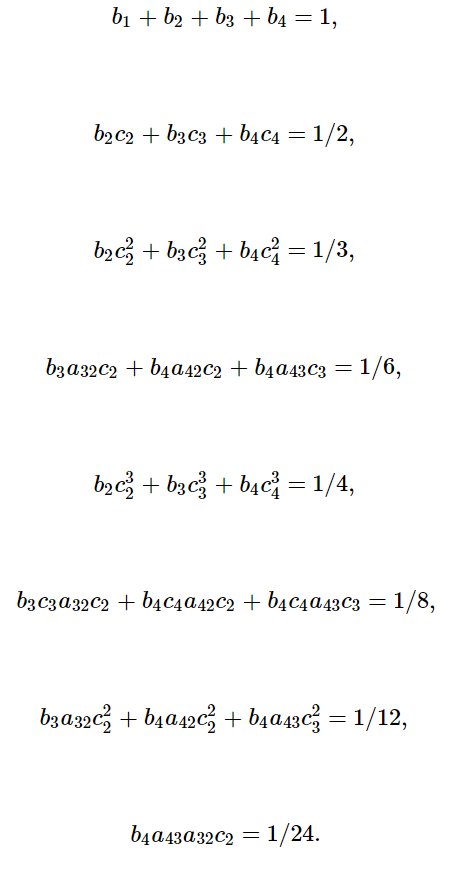
The classic Runge-Kutta method is also known as RK4 and is the following 4th order method:
\[ k_1 = f(u_n,p,t)\\ k_2 = f(u_n + \frac{\Delta t}{2} k_1,p,t + \frac{\Delta t}{2})\\ k_3 = f(u_n + \frac{\Delta t}{2} k_2,p,t + \frac{\Delta t}{2})\\ k_4 = f(u_n + \Delta t k_3,p,t + \Delta t)\\ u_{n+1} = u_n + \frac{\Delta t}{6}(k_1 + 2 k_2 + 2 k_3 + k_4)\\ \]
While it's widely known and simple to remember, it's not necessarily good. The way to judge a Runge-Kutta method is by looking at the size of the coefficient of the next term in the Taylor series: if it's large then the true error can be larger, even if it matches another one asymptotically.
What Makes a Good Method?
Leading Truncation Coefficients
For given orders of explicit Runge-Kutta methods, lower bounds for the number of f evaluations (stages) required to receive a given order are known:
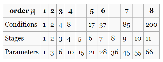
While unintuitive, using the method is not necessarily the one that reduces the coefficient the most. The reason is because what is attempted in ODE solving is precisely the opposite of the analysis. In the ODE analysis, we're looking at behavior as $\Delta t \rightarrow 0$. However, when efficiently solving ODEs, we want to use the largest $\Delta t$ which satisfies error tolerances.
The most widely used method is the Dormand-Prince 5th order Runge-Kutta method, whose tableau is represented as:

Notice that this method takes 7 calls to f for 5th order. The key to this method is that it has optimized leading truncation error coefficients, under some extra assumptions which allow for the analysis to be simplified.
Looking at the Effects of RK Method Choices and Code Optimizations
Pulling from the SciML Benchmarks, we can see the general effect of these different properties on a given set of Runge-Kutta methods:
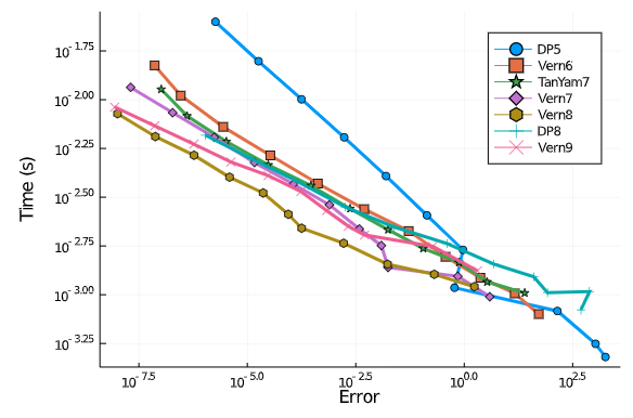
Here, the order of the method is given in the name. We can see one immediate factor is that, as the requested error in the calculation decreases, the higher order methods become more efficient. This is because to decrease error, you decrease $\Delta t$, and thus the exponent difference with respect to $\Delta t$ has more of a chance to pay off for the extra calls to f. Additionally, we can see that order is not the only determining factor for efficiency: the Vern8 method seems to have a clear approximate 2.5x performance advantage over the whole span of the benchmark compared to the DP8 method, even though both are 8th order methods. This is because of the leading truncation terms: with a small enough $\Delta t$, the more optimized method (Vern8) will generally have low error in a step for the same $\Delta t$ because the coefficients in the expansion are generally smaller.
This is a factor which is generally ignored in high level discussions of numerical differential equations, but can lead to orders of magnitude differences! This is highlighted in the following plot:
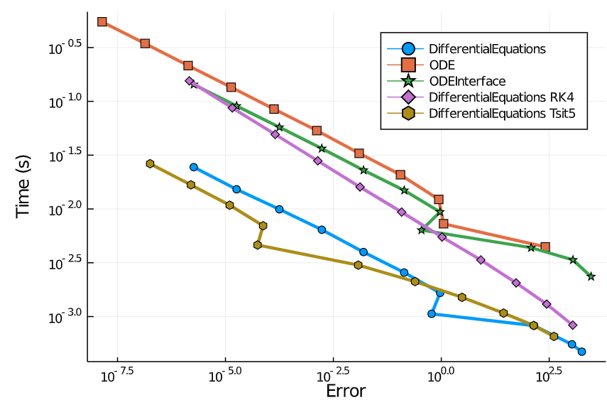
Here we see ODEInterface.jl's ODEInterfaceDiffEq.jl wrapper into the SciML common interface for the standard dopri method from Fortran, and ODE.jl, the original ODE solvers in Julia, have a performance disadvantage compared to the DifferentialEquations.jl methods due in part to some of the coding performance pieces that we discussed in the first few lectures.
Specifically, a large part of this can be attributed to inlining of the higher order functions, i.e. ODEs are defined by a user function and then have to be called from the solver. If the solver code is compiled as a shared library ahead of time, like is commonly done in C++ or Fortran, then there can be a function call overhead that is eliminated by JIT compilation optimizing across the function call barriers (known as interprocedural optimization). This is one way which a JIT system can outperform an AOT (ahead of time) compiled system in real-world code (for completeness, two other ways are by doing full function specialization, which is something that is not generally possible in AOT languages given that you cannot know all types ahead of time for a fully generic function, and calling C itself, i.e. c-ffi (foreign function interface), can be optimized using the runtime information of the JIT compiler to outperform C!).
The other performance difference being shown here is due to optimization of the method. While a slightly different order, we can see a clear difference in the performance of RK4 vs the coefficient optimized methods. It's about the same order of magnitude as "highly optimized code differences", showing that both the Runge-Kutta coefficients and the code implementation can have a significant impact on performance.
Taking a look at what happens when interpreted languages get involved highlights some of the code challenges in this domain. Let's take a look at for example the results when simulating 3 ODE systems with the various RK methods:
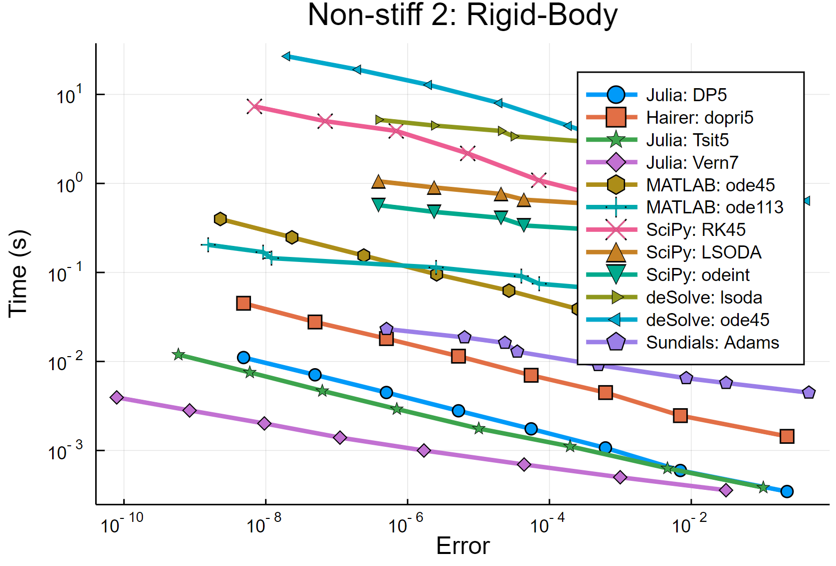
We see that using interpreted languages introduces around a 50x-100x performance penalty. If you recall in your previous lecture, the discrete dynamical system that was being simulated was the 3-dimensional Lorenz equation discretized by Euler's method, meaning that the performance of that implementation is a good proxy for understanding the performance differences in this graph. Recall that in previous lectures we saw an approximately 5x performance advantage when specializing on the system function and size and around 10x by reducing allocations: these features account for the performance differences noticed between library implementations, which are then compounded by the use of different RK methods (note that R uses "call by copy" which even further increases the memory usages and makes standard usage of the language incompatible with mutating function calls!).
Stability of a Method
Simply having an order on the truncation error does not imply convergence of the method. The disconnect is that the errors at a given time point may not dissipate. What also needs to be checked is the asymptotic behavior of a disturbance. To see this, one can utilize the linear test problem:
\[ u' = \alpha u \]
and ask the question, does the discrete dynamical system defined by the discretized ODE end up going to zero? You would hope that the discretized dynamical system and the continuous dynamical system have the same properties in this simple case, and this is known as linear stability analysis of the method.
As an example, take a look at the Euler method. Recall that the Euler method was given by:
\[ u_{n+1} = u_n + \Delta t f(u_n,p,t) \]
When we plug in the linear test equation, we get that
\[ u_{n+1} = u_n + \Delta t \alpha u_n \]
If we let $z = \Delta t \alpha$, then we get the following:
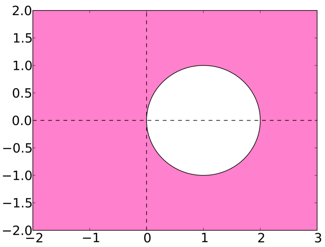
\[ u_{n+1} = u_n + z u_n = (1+z)u_n \]
which is stable when $z$ is in the shifted unit circle. This means that, as a necessary condition, the step size $\Delta t$ needs to be small enough that $z$ satisfies this condition, placing a stepsize limit on the method.
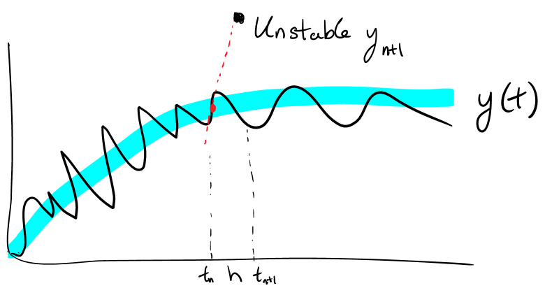
If $\Delta t$ is ever too large, it will cause the equation to overshoot zero, which then causes oscillations that spiral out to infinity.
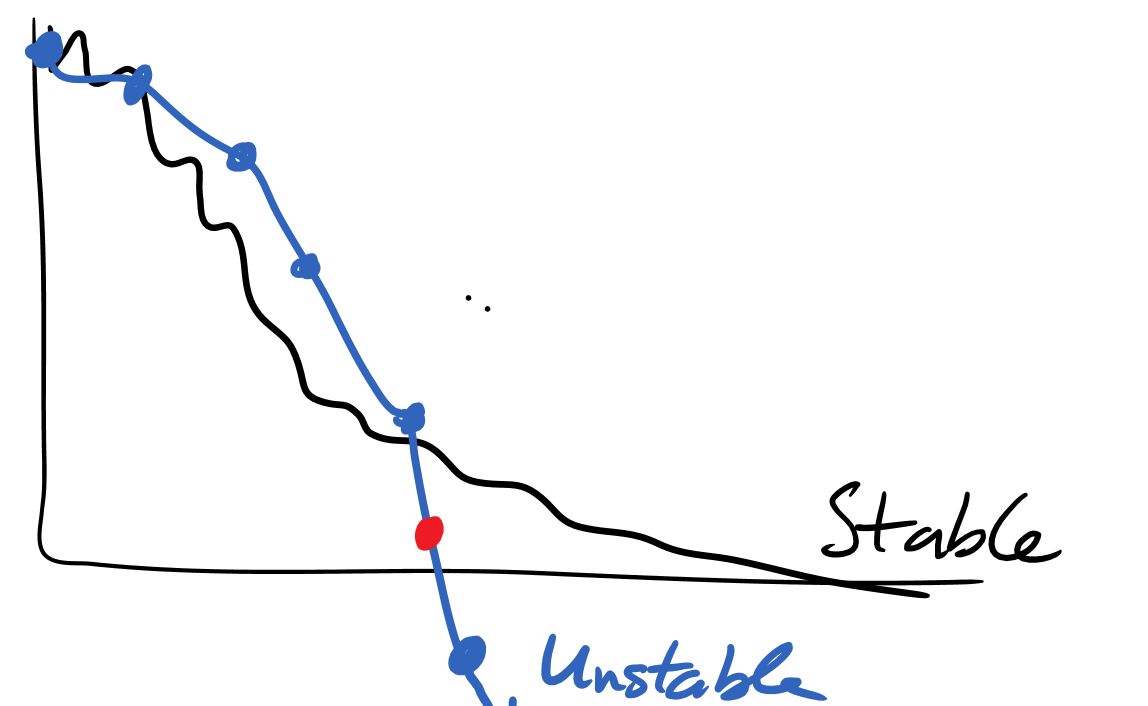
Thus the stability condition places a hard constraint on the allowed $\Delta t$ which will result in a realistic simulation.
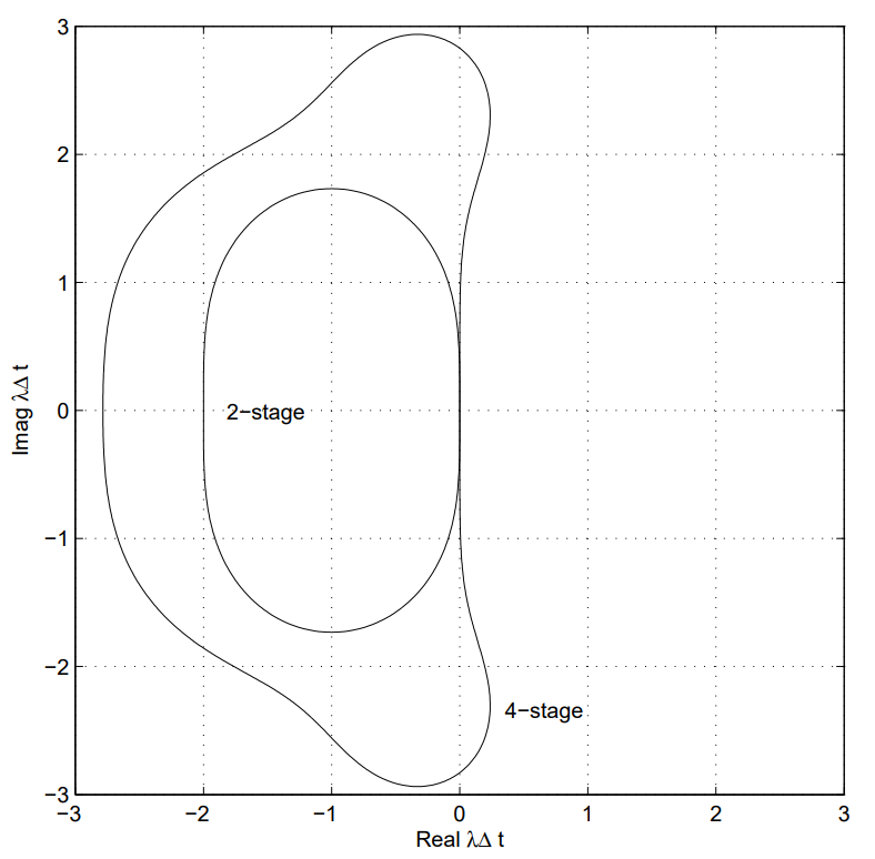
For reference, the stability regions of the 2nd and 4th order Runge-Kutta methods that we discussed are as follows:
Interpretation of the Linear Stability Condition
To interpret the linear stability condition, recall that the linearization of a system interprets the dynamics as locally being due to the Jacobian of the system. Thus
\[ u' = f(u,p,t) \]
is locally equivalent to
\[ u' = \frac{df}{du}u \]
You can understand the local behavior through diagonalizing this matrix. Therefore, the scalar for the linear stability analysis is performing an analysis on the eigenvalues of the Jacobian. The method will be stable if the largest eigenvalues of df/du are all within the stability limit. This means that stability effects are different throughout the solution of a nonlinear equation and are generally understood locally (though different more comprehensive stability conditions exist!).
Implicit Methods
If instead of the Euler method we defined $f$ to be evaluated at the future point, we would receive a method like:
\[ u_{n+1} = u_n + \Delta t f(u_{n+1},p,t+\Delta t) \]
in which case, for the stability calculation we would have that
\[ u_{n+1} = u_n + \Delta t \alpha u_n \]
or
\[ (1-z) u_{n+1} = u_n \]
which means that
\[ u_{n+1} = \frac{1}{1-z} u_n \]
which is stable for all $Re(z) < 0$ a property which is known as A-stability. It is also stable as $z \rightarrow \infty$, a property known as L-stability. This means that for equations with very ill-conditioned Jacobians, this method is still able to be use reasonably large stepsizes and can thus be efficient.
Stiffness and Timescale Separation
From this we see that there is a maximal stepsize whenever the eigenvalues of the Jacobian are sufficiently large. It turns out that's not an issue if the phenomena we see are fast, since then the total integration time tends to be small. However, if we have some equations with both fast modes and slow modes, like the Robertson equation, then it is very difficult because in order to resolve the slow dynamics over a long timespan, one needs to ensure that the fast dynamics do not diverge. This is a property known as stiffness. Stiffness can thus be approximated in some sense by the condition number of the Jacobian. The condition number of a matrix is its maximal eigenvalue divided by its minimal eigenvalue and gives a rough measure of the local timescale separations. If this value is large and one wants to resolve the slow dynamics, then explicit integrators, like the explicit Runge-Kutta methods described before, have issues with stability. In this case implicit integrators (or other forms of stabilized stepping) are required in order to efficiently reach the end time step.
Exploiting Continuity
So far, we have looked at ordinary differential equations as a $\Delta t \rightarrow 0$ formulation of a discrete dynamical system. However, continuous dynamics and discrete dynamics have very different characteristics which can be utilized in order to arrive at simpler models and faster computations.
Geometric Properties: No Jumping and the Poincaré–Bendixson theorem
In terms of geometric properties, continuity places a large constraint on the possible dynamics. This is because of the physical constraint on "jumping", i.e. flows of differential equations cannot jump over each other. If you are ever at some point in phase space and $f$ is not explicitly time-dependent, then the direction of $u'$ is uniquely determined (given reasonable assumptions on $f$), meaning that flow lines (solutions to the differential equation) can never cross.
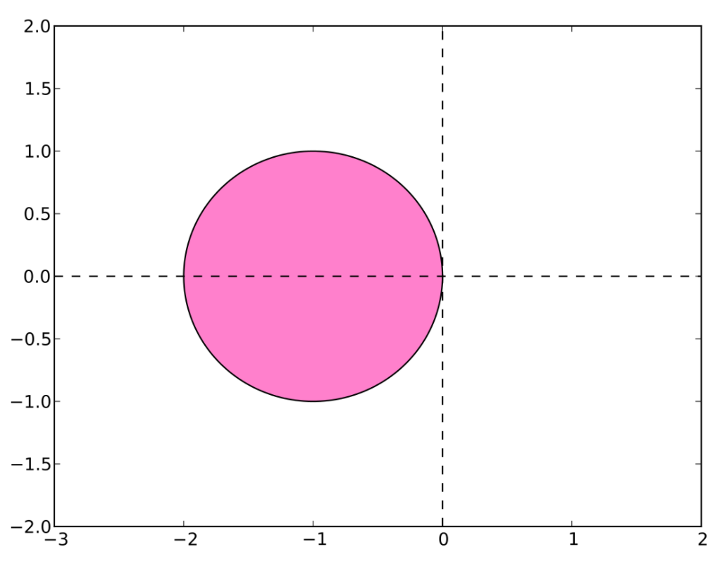
A result from this is the Poincaré–Bendixson theorem, which states that, with any arbitrary (but nice) two dimensional continuous system, you can only have 3 behaviors:
Steady state behavior
Divergence
Periodic orbits
A simple proof by picture shows this.