Solving Stiff Ordinary Differential Equations
Chris Rackauckas
October 14th, 2020
Youtube Video Link
We have previously shown how to solve non-stiff ODEs via optimized Runge-Kutta methods, but we ended by showing that there is a fundamental limitation of these methods when attempting to solve stiff ordinary differential equations. However, we can get around these limitations by using different types of methods, like implicit Euler. Let's now go down the path of understanding how to efficiently implement stiff ordinary differential equation solvers, and its interaction with other domains like automatic differentiation.
When one is solving a large-scale scientific computing problem with MPI, this is almost always the piece of code where all of the time is spent, so let's understand how what it's doing.
Newton's Method and Jacobians
Recall that the implicit Euler method is the following:
\[ u_{n+1} = u_n + \Delta t f(u_{n+1},p,t + \Delta t) \]
If we wanted to use this method, we would need to find out how to get the value $u_{n+1}$ when only knowing the value $u_n$. To do so, we can move everything to one side:
\[ u_{n+1} - \Delta t f(u_{n+1},p,t + \Delta t) - u_n = 0 \]
and now we have a problem
\[ g(u_{n+1}) = 0 \]
This is the classic rootfinding problem $g(x)=0$, find $x$. The way that we solve the rootfinding problem is, once again, by replacing this problem about a continuous function $g$ with a discrete dynamical system whose steady state is the solution to the $g(x)=0$. There are many methods for this, but some choices of the rootfinding method effect the stability of the ODE solver itself since we need to make sure that the steady state solution is a stable steady state of the iteration process, otherwise the rootfinding method will diverge (will be explored in the homework).
Thus for example, fixed point iteration is not appropriate for stiff differential equations. Methods which are used in the stiff case are either Anderson Acceleration or Newton's method. Newton's is by far the most common (and generally performs the best), so we can go down this route.
Let's use the syntax $g(x)=0$. Here we need some starting value $x_0$ as our first guess for $u_{n+1}$. The easiest guess is $u_{n}$, though additional information about the equation can be used to compute a better starting value (known as a step predictor). Once we have a starting value, we run the iteration:
\[ x_{k+1} = x_k - J(x_k)^{-1}g(x_k) \]
where $J(x_k)$ is the Jacobian of $g$ at the point $x_k$. However, the mathematical formulation is never the syntax that you should use for the actual application! Instead, numerically this is two stages:
Solve $Ja=g(x_k)$ for $a$
Update $x_{k+1} = x_k - a$
By doing this, we can turn the matrix inversion into a problem of a linear solve and then an update. The reason this is done is manyfold, but one major reason is because the inverse of a sparse matrix can be dense, and this Jacobian is in many cases (PDEs) a large and dense matrix.
Now let's break this down step by step.
Some Quick Notes
The Jacobian of $g$ can also be written as $J = I - \gamma \frac{df}{du}$ for the ODE $u' = f(u,p,t)$, where $\gamma = \Delta t$ for the implicit Euler method. This general form holds for all other (SDIRK) implicit methods, changing the value of $\gamma$. Additionally, the class of Rosenbrock methods solves a linear system with exactly the same $J$, meaning that essentially all implicit and semi-implicit ODE solvers have to do the same Newton iteration process on the same structure. This is the portion of the code that is generally the bottleneck.
Additionally, if one is solving a mass matrix ODE: $Mu' = f(u,p,t)$, exactly the same treatment can be had with $J = M - \gamma \frac{df}{du}$. This works even if $M$ is singular, a case known as a differential-algebraic equation or a DAE. A DAE for example can be an ODE with constraint equations, and these structures can be represented as an ODE where these constraints lead to a singularity in the mass matrix (a row of all zeros is a term that is only the right hand side equals zero!).
Generation of the Jacobian
Dense Finite Differences and Forward-Mode AD
Recall that the Jacobian is the matrix of $\frac{df_i}{dx_j}$ for $f$ a vector-valued function. The simplest way to generate the Jacobian is through finite differences. For each $h_j = h e_j$ for $e_j$ the basis vector of the $j$th axis and some sufficiently small $h$, then we can compute column $j$ of the Jacobian by:
\[ \frac{f(x+h_j)-f(x)}{h} \]
Thus $m+1$ applications of $f$ are required to compute the full Jacobian.
This can be improved by using forward-mode automatic differentiation. Recall that we can formulate a multidimensional duel number of the form
\[ d = x + v_1 \epsilon_1 + \ldots + v_m \epsilon_m \]
We can then seed the vectors $v_j = h_j$ so that the differentiation directions are along the basis vectors, and then the output dual is the result:
\[ f(d) = f(x) + J_1 \epsilon_1 + \ldots + J_m \epsilon_m \]
where $J_j$ is the $j$th column of the Jacobian. And thus with one calculation of the primal (f(x)) we have calculated the entire Jacobian.
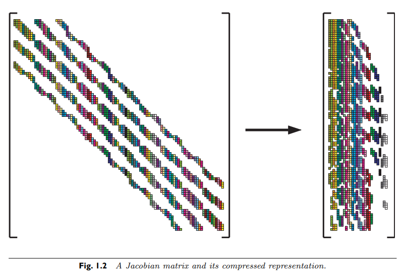
Sparse Differentiation and Matrix Coloring
However, when the Jacobian is sparse we can compute it much faster. We can understand this by looking at the following system:
\[ f(x)=\left[\begin{array}{c} x_{1}+x_{3}\\ x_{2}x_{3}\\ x_{1} \end{array}\right] \]
Notice that in 3 differencing steps we can calculate:
\[ f(x+\epsilon e_{1})=\left[\begin{array}{c} x_{1}+x_{3}+\epsilon\\ x_{2}x_{3}\\ x_{1}+\epsilon \end{array}\right] \]
\[ f(x+\epsilon e_{2})=\left[\begin{array}{c} x_{1}+x_{3}\\ x_{2}x_{3}+\epsilon x_{3}\\ x_{1} \end{array}\right] \]
\[ f(x+\epsilon e_{3})=\left[\begin{array}{c} x_{1}+x_{3}+\epsilon\\ x_{2}x_{3}+\epsilon x_{2}\\ x_{1} \end{array}\right] \]
and thus:
\[ \frac{f(x+\epsilon e_{1})-f(x)}{\epsilon}=\left[\begin{array}{c} 1\\ 0\\ 1 \end{array}\right] \]
\[ \frac{f(x+\epsilon e_{2})-f(x)}{\epsilon}=\left[\begin{array}{c} 0\\ x_{3}\\ 0 \end{array}\right] \]
\[ \frac{f(x+\epsilon e_{3})-f(x)}{\epsilon}=\left[\begin{array}{c} 1\\ x_{2}\\ 0 \end{array}\right] \]
But notice that the calculation of $e_1$ and $e_2$ do not interact. If we had done:
\[ \frac{f(x+\epsilon e_{1}+\epsilon e_{2})-f(x)}{\epsilon}=\left[\begin{array}{c} 1\\ x_{3}\\ 1 \end{array}\right] \]
we would still get the correct value for every row because the $\epsilon$ terms do not collide (a situation known as perturbation confusion). If we knew the sparsity pattern of the Jacobian included a 0 at (2,1), (1,2), and (3,2), then we would know that the vectors would have to be $[1 0 1]$ and $[0 x_3 0]$, meaning that columns 1 and 2 can be computed simultaneously and decompressed. This is the key to sparse differentiation.
With forward-mode automatic differentiation, recall that we calculate multiple dimensions simultaneously by using a multidimensional dual number seeded by the vectors of the differentiation directions, that is:
\[ d = x + v_1 \epsilon_1 + \ldots + v_m \epsilon_m \]
Instead of using the primitive differentiation directions $e_j$, we can instead replace this with the mixed values. For example, the Jacobian of the example function can be computed in one function call to $f$ with the dual number input:
\[ d = x + (e_1 + e_2) \epsilon_1 + e_3 \epsilon_2 \]
and performing the decompression via the sparsity pattern. Thus the sparsity pattern gives a direct way to optimize the construction of the Jacobian.
This idea of independent directions can be formalized as a matrix coloring. Take $S_{ij}$ the sparsity pattern of some Jacobian matrix $J_{ij}$. Define a graph on the nodes 1 through m where there is an edge between $i$ and $j$ if there is a row where $i$ and $j$ are non-zero. This graph is the column connectivity graph of the Jacobian. What we wish to do is find the smallest set of differentiation directions such that differentiating in the direction of $e_i$ does not collide with differentiation in the direction of $e_j$. The connectivity graph is setup so that way this cannot be done if the two nodes are adjacent. If we let the subset of nodes differentiated together be a color, the question is, what is the smallest number of colors s.t. no adjacent nodes are the same color. This is the classic distance-1 coloring problem from graph theory. It is well-known that the problem of finding the chromatic number, the minimal number of colors for a graph, is generally NP-complete. However, there are heuristic methods for performing a distance-1 coloring quite quickly. For example, a greedy algorithm is as follows:
Pick a node at random to be color 1.
Make all nodes adjacent to that be the lowest color that they can be (in this step that will be 2).
Now look at all nodes adjacent to that. Make all nodes be the lowest color that they can be (either 1 or 3).
Repeat by looking at the next set of adjacent nodes and color as conservatively as possible.
This can be visualized as follows:
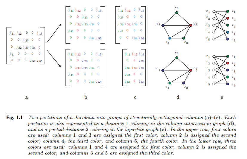
The result will color the entire connected component. While not giving an optimal result, it will still give a result that is a sufficient reduction in the number of differentiation directions (without solving an NP-complete problem) and thus can lead to a large computational saving.
At the end, let $c_i$ be the vector of 1's and 0's, where it's 1 for every node that is color $i$ and 0 otherwise. Sparse automatic differentiation of the Jacobian is then computed with:
\[ d = x + c_1 \epsilon_1 + \ldots + c_k \epsilon_k \]
that is, the full Jacobian is computed with one dual number which consists of the primal calculation along with $k$ dual dimensions, where $k$ is the computed chromatic number of the connectivity graph on the Jacobian. Once this calculation is complete, the colored columns can be decompressed into the full Jacobian using the sparsity information, generating the original quantity that we wanted to compute.
For more information on the graph coloring aspects, find the paper titled "What Color Is Your Jacobian? Graph Coloring for Computing Derivatives" by Gebremedhin.
Note on Sparse Reverse-Mode AD
Reverse-mode automatic differentiation can be though of as a method for computing one row of a Jacobian per seed, as opposed to one column per seed given by forward-mode AD. Thus sparse reverse-mode automatic differentiation can be done by looking at the connectivity graph of the column and using the resulting color vectors to seed the reverse accumulation process.
Linear Solving
After the Jacobian has been computed, we need to solve a linear equation $Ja=b$. While mathematically you can solve this by computing the inverse $J^{-1}$, this is not a good way to perform the calculation because even if $J$ is sparse, then $J^{-1}$ is in general dense and thus may not fit into memory (remember, this is $N^2$ as many terms, where $N$ is the size of the ordinary differential equation that is being solved, so if it's a large equation it is very feasible and common that the ODE is representable but its full Jacobian is not able to fit into RAM). Note that some may say that this is done for numerical stability reasons: that is incorrect. In fact, under reasonable assumptions for how the inverse is computed, it will be as numerically stable as other techniques we will mention.
Thus instead of generating the inverse, we can instead perform a matrix factorization. A matrix factorization is a transformation of the matrix into a form that is more amenable to certain analyses. For our purposes, a general Jacobian within a Newton iteration can be transformed via the LU-factorization or (LU-decomposition), i.e.
\[ J = LU \]
where $L$ is lower triangular and $U$ is upper triangular. If we write the linear equation in this form:
\[ LUa = b \]
then we see that we can solve it by first solving $L(Ua) = b$. Since $L$ is lower triangular, this is done by the backsubstitution algorithm. That is, in a lower triangular form, we can solve for the first value since we have:
\[ L_{11} a_1 = b_1 \]
and thus by dividing we solve. For the next term, we have that
\[ L_{21} a_1 + L_{22} a_2 = b_2 \]
and thus we plug in the solution to $a_1$ and solve to get $a_2$. The lower triangular form allows this to continue. This occurs in 1+2+3+...+n operations, and is thus O(n^2). Next, we solve $Ua = b$, which once again is done by a backsubstitution algorithm but in the reverse direction. Together those two operations are O(n^2) and complete the inversion of $LU$.
So is this an O(n^2) algorithm for computing the solution of a linear system? No, because the computation of $LU$ itself is an O(n^3) calculation, and thus the true complexity of solving a linear system is still O(n^3). However, if we have already factorized $J$, then we can repeatedly use the same $LU$ factors to solve additional linear problems $Jv = u$ with different vectors. We can exploit this to accelerate the Newton method. Instead of doing the calculation:
\[ x_{k+1} = x_k - J(x_k)^{-1}g(x_k) \]
we can instead do:
\[ x_{k+1} = x_k - J(x_0)^{-1}g(x_k) \]
so that all of the Jacobians are the same. This means that a single O(n^3) factorization can be done, with multiple O(n^2) calculations using the same factorization. This is known as a Quasi-Newton method. While this makes the Newton method no longer quadratically convergent, it minimizes the large constant factor on the computational cost while retaining the same dynamical properties, i.e. the same steady state and thus the same overall solution. This makes sense for sufficiently large $n$, but requires sufficiently large $n$ because the loss of quadratic convergence means that it will take more steps to converge than before, and thus more $O(n^2)$ backsolves are required, meaning that the difference between factorizations and backsolves needs to be large enough in order to offset the cost of extra steps.
Note on Sparse Factorization
Note that LU-factorization, and other factorizations, have generalizations to sparse matrices where a symbolic factorization is utilized to compute a sparse storage of the values which then allow for a fast backsubstitution. More details are outside the scope of this course, but note that Julia and MATLAB will both use the library SuiteSparse in the background when lu is called on a sparse matrix.
Jacobian-Free Newton Krylov (JFNK)
An alternative method for solving the linear system is the Jacobian-Free Newton Krylov technique. This technique is broken into two pieces: the jvp calculation and the Krylov subspace iterative linear solver.
Jacobian-Vector Products as Directional Derivatives
We don't actually need to compute $J$ itself, since all that we actually need is the v = J*w. Is it possible to compute the Jacobian-Vector Product, or the jvp, without producing the Jacobian?
To see how this is done let's take a look at what is actually calculated. Written out in the standard basis, we have that:
\[ w_i = \sum_{j}^{m} J_{ij} v_{j} \]
Now write out what $J$ means and we see that:
\[ w_i = \sum_j^{m} \frac{df_i}{dx_j} v_j = \nabla f_i(x) \cdot v \]
that is, the $i$th component of $Jv$ is the directional derivative of $f_i$ in the direction $v$. This means that in general, the jvp $Jv$ is actually just the directional derivative in the direction of $v$, that is:
\[ Jv = \nabla f \cdot v \]
and therefore it has another mathematical representation, that is:
\[ Jv = \lim_{\epsilon \rightarrow 0} \frac{f(x+v \epsilon) - f(x)}{\epsilon} \]
From this alternative form it is clear that we can always compute a jvp with a single computation. Using finite differences, a simple approximation is the following:
\[ Jv \approx \frac{f(x+v \epsilon) - f(x)}{\epsilon} \]
for non-zero $\epsilon$. Similarly, recall that in forward-mode automatic differentiation we can choose directions by seeding the dual part. Therefore, using the dual number with one partial component:
\[ d = x + v \epsilon \]
we get that
\[ f(d) = f(x) + Jv \epsilon \]
and thus a single application with a single partial gives the jvp.
Note on Reverse-Mode Automatic Differentiation
As noted earlier, reverse-mode automatic differentiation has its primitives compute rows of the Jacobian in the seeded direction. This means that the seeded reverse-mode call with the vector $v$ computes $v^T J$, that is the vector (transpose) Jacobian transpose, or vjp for short. When discussing parameter estimation and adjoints, this shorthand will be introduced as a way for using a traditionally machine learning tool to accelerate traditionally scientific computing tasks.
Krylov Subspace Methods For Solving Linear Systems
Basic Iterative Solver Methods
Now that we have direct access to quick calculations of $Jv$, how would we use this to solve the linear system $Jw = v$ quickly? This is done through iterative linear solvers. These methods replace the process of solving for a factorization with, you may have guessed it, a discrete dynamical system whose solution is $w$. To do this, what we want is some iterative process so that
\[ Jw - b = 0 \]
So now let's split $J = A - B$, then if we are iterating the vectors $w_k$ such that $w_k \rightarrow w$, then if we plug this into the previous (residual) equation we get
\[ A w_{k+1} = Bw_k + b \]
since when we plug in $w$ we get zero (the sequence must be Cauchy so the difference $w_{k+1} - w_k \rightarrow 0$). Thus if we can split our matrix $J$ into a component $A$ which is easy to invert and a part $B$ that is just everything else, then we would have a bunch of easy linear systems to solve. There are many different choices that we can do. If we let $J = L + D + U$, where $L$ is the lower portion of $J$, $D$ is the diagonal, and $U$ is the upper portion, then the following are well-known methods:
Richardson: $A = \omega I$ for some $\omega$
Jacobi: $A = D$
Damped Jacobi: $A = \omega D$
Gauss-Seidel: $A = D-L$
Successive Over Relaxation: $A = \omega D - L$
Symmetric Successive Over Relaxation: $A = \frac{1}{\omega (2 - \omega)}(D-\omega L)D^{-1}(D-\omega U)$
These decompositions are chosen since a diagonal matrix is easy to invert (it's just the inversion of the scalars of the diagonal) and it's easy to solve an upper or lower triangular linear system (once again, it's backsubstitution).
Since these methods give a a linear dynamical system, we know that there is a unique steady state solution, which happens to be $Aw - Bw = Jw = b$. Thus we will converge to it as long as the steady state is stable. To see if it's stable, take the update equation
\[ w_{k+1} = A^{-1}(Bw_k + b) \]
and check the eigenvalues of the system: if they are within the unit circle then you have stability. Notice that this can always occur by bringing the eigenvalues of $A^{-1}$ closer to zero, which can be done by multiplying $A$ by a significantly large value, hence the $\omega$ quantities. While that always works, this essentially amounts to decreasing the stepsize of the iterative process and thus requiring more steps, thus making it take more computations. Thus the game is to pick the largest stepsize ($\omega$) for which the steady state is stable. We will leave that as outside the topic of this course.
Krylov Subspace Methods
While the classical iterative solver methods give the background for understanding an alternative to direct inversion or factorization of a matrix, the problem with that approach is that it requires the ability to split the matrix $J$, which we would like to avoid computing. Instead, we would like to develop an iterative solver technique which instead just uses the solution to $Jv$. Indeed there are such methods, and these are the Krylov subspace methods. A Krylov subspace is the space spanned by:
\[ \mathcal{K}_k = \text{span} \{v,Jv,J^2 v, \ldots, J^k v\} \]
There are a few nice properties about Krylov subspaces that can be exploited. For one, it is known that there is a finite maximum dimension of the Krylov subspace, that is there is a value $r$ such that $J^{r+1} v \in \mathcal{K}_r$, which means that the complete Krylov subspace can be computed in finitely many jvp, since $J^2 v$ is just the jvp where the vector is the jvp. Indeed, one can show that $J^i v$ is linearly independent for each $i$, and thus that maximal value is $m$, the dimension of the Jacobian. Therefore in $m$ jvps the solution is guaranteed to live in the Krylov subspace, giving a maximal computational cost and a proof of convergence if the vector in there is the "optimal in the space".
The most common method in the Krylov subspace family of methods is the GMRES method. Essentially, in step $i$ one computes $\mathcal{K}_i$, and finds the $x$ that is the closest to the Krylov subspace, i.e. finds the $x \in \mathcal{K}_i$ such that $\Vert Jx-v \Vert_2$ is minimized. At each step, it adds the new vector to the Krylov subspace after orthogonalizing it against the other vectors via Arnoldi iterations, leading to an orthogonal basis of $\mathcal{K}_i$ which makes it easy to express $x$.
While one has a guaranteed bound on the number of possible jvps in GMRES which is simply the number of ODEs (since that is what determines the size of the Jacobian and thus the total dimension of the problem), that bound is not necessarily a good one. For a large sparse matrix, it may be computationally impractical to ever compute 100,000 jvps. Thus one does not typically run the algorithm to conclusion, and instead stops when $\Vert Jx-v \Vert-2$ is sufficiently below some user-defined error tolerance.
Intermediate Conclusion
Let's take a step back and see what our intermediate conclusion is. In order to solve for the implicit step, it just boils down to doing Newton's method on some $g(x)=0$. If the Jacobian is small enough, one factorizes the Jacobian and uses Quasi-Newton iterations in order to utilize the stored LU-decomposition in multiple steps to reduce the computation cost. If the Jacobian is sparse, sparse automatic differentiation through matrix coloring is employed to directly fill the sparse matrix with less applications of $g$, and then this sparse matrix is factorized using a sparse LU factorization.
When the matrix is too large, then one resorts to using a Krylov subspace method, since this only requires being able to do $Jv$ calculations. In general, $Jv$ can be done matrix-free because it is simply the directional derivative in the direction of the vector $v$, which can be computed through either numerical or forward-mode automatic differentiation. This is then used in the GMRES iterative process to find the solution in the Krylov subspace which is closest to the solution, exiting early when the residual error is small enough. If this is converging too slow, then preconditioning is used.
That's the basic algorithm, but what are the other important details for getting this right?
The Need for Speed
Preconditioning
However, the speed at GMRES convergences is dependent on the correlations between the vectors, which can be shown to be related to the condition number of the Jacobian matrix. A high condition number makes convergence slower (this is the case for the traditional iterative methods as well), which in turn is an issue because it is the high condition number on the Jacobian which leads to stiffness and causes one to have to use an implicit integrator in the first place!
To help speed up the convergence, a common technique is known as preconditioning. Preconditioning is the process of using a semi-inverse to the matrix in order to split the matrix so that the iterative problem that is being solved is one that has a smaller condition number. Mathematically, it involves decomposing $J = P_l A P_r$ where $P_l$ and $P_r$ are the left and right preconditioners which have simple inverses, and thus instead of solving $Jx=v$, we would solve:
\[ P_l A P_r x = v \]
or
\[ A P_r x = P_l^{-1}v \]
which then means that the Krylov subpace that needs to be solved for is that defined by $A$: $\mathcal{K} = \text{span}\{v,Av,A^2 v, \ldots\}$. There are many possible choices for these preconditioners, but they are usually problem dependent. For example, for ODEs which come from parabolic and elliptic PDE discretizations, the multigrid method, such as a geometric multigrid or an algebraic multigrid, is a preconditioner that can accelerate the iterative solving process. One generic preconditioner that can generally be used is to divide by the norm of the vector $v$, which is a scaling employed by both SUNDIALS CVODE and by DifferentialEquations.jl and can be shown to be almost always advantageous.
Jacobian Re-use
If the problem is small enough such that the factorization is used and a Quasi-Newton technique is employed, it then holds that for most steps $J$ is only approximate since it can be using an old LU-factorization. To push it even further, high performance codes allow for jacobian reuse, which is allowing the same Jacobian to be reused between different timesteps. If the Jacobian is too incorrect, it can cause the Newton iterations to diverge, which is then when one would calculate a new Jacobian and compute a new LU-factorization.
Adaptive Timestepping
In simple cases, like partial differential equation discretizations of physical problems, the resulting ODEs are not too stiff and thus Newton's iteration generally works. However, in cases like stiff biological models, Newton's iteration can itself not always be stable enough to allow convergence. In fact, with many of the stiff biological models commonly used in benchmarks, no method is stable enough to pass without using adaptive timestepping! Thus one may need to adapt the timestep in order to improve the ability for the Newton method to converge (smaller timesteps increase the stability of the Newton stepping, see the homework).
This needs to be mixed with the Jacobian re-use strategy, since $J = I - \gamma \frac{df}{du}$ where $\gamma$ is dependent on $\Delta t$ (and $\gamma = \Delta t$ for implicit Euler) means that the Jacobian of the Newton method changes as $\Delta t$ changes. Thus one usually has a tiered algorithm for determining when to update the factorizations of $J$ vs when to compute a new $\frac{df}{du}$ and then refactorize. This is generally dependent on estimates of convergence rates to heuristically guess how far off $\frac{df}{du}$ is from the current true value.
So how does one perform adaptivity? This is generally done through a rejection sampling technique. First one needs some estimate of the error in a step. This is calculated through an embedded method, which is a method that is able to be calculated without any extra $f$ evaluations that is (usually) one order different from the true method. The difference between the true and the embedded method is then an error estimate. If this is greater than a user chosen tolerance, the step is rejected and re-ran with a smaller $\Delta t$ (possibly refactorizing, etc.). If this is less than the user tolerance, the step is accepted and $\Delta t$ is changed.
There are many schemes for how one can change $\Delta t$. One of the most common is known as the P-control, which stands for the proportional controller which is used throughout control theory. In this case, the control is to change $\Delta t$ in proportion to the current error ratio from the desired tolerance. If we let $\text{E}$ be the error estimate (the difference between the true and embedded method), and
\[ q = \frac{\text{E}}{\max(u_k,u_{k+1}) \tau_r + \tau_a} \]
where $\tau_r$ is the relative tolerance and $\tau_a$ is the absolute tolerance, then $q$ is the ratio of the current error to the current tolerance. If $q<1$, then the error is less than the tolerance and the step is accepted, and vice versa for $q>1$. In either case, we let $\Delta t_{new} = q \Delta t$ be the proportional update.
However, proportional error control has many known features that are undesirable. For example, it happens to work in a "bang bang" manner, meaning that it can drastically change its behavior from step to step. One step may multiply the step size by 10x, then the next by 2x. This is an issue because it effects the stability of the ODE solver method (since the stability is not a property of a single step, but rather it's a property of the global behavior over time)! Thus to smooth it out, one can use a PI-control, which modifies the control factor by a history value, i.e. the error in one step in the past. This of course also means that one can utilize a PID-controller for time stepping. And there are many other techniques that can be used, but many of the most optimized codes tend to use a PI-control mechanism.
Methodological Summary
Here's a quick summary of the methodologies in a hierarchical sense:
At the lowest level is the linear solve, either done by JFNK or (sparse) factorization. For large enough systems, this is the brunt of the work. This is thus the piece to computationally optimize as much as possible, and parallelize. For sparse factorizations, this can be done with a distributed sparse library implementation. For JFNK, the efficiency is simply due to the efficiency of your ODE function
f.An optional level for JFNK is the preconditioning level, where preconditioners can be used to decrease the total number of iterations required for Krylov subspace methods like GMRES to converge, and thus reduce the total number of
fcalls.At the nonlinear solver level, different Newton-like techniques are utilized to minimize the number of factorizations/linear solves required, and maximize the stability of the Newton method.
At the ODE solver level, more efficient integrators and adaptive methods for stiff ODEs are used to reduce the cost by affecting the linear solves. Most of these calculations are dominated by the linear solve portion when it's in the regime of large stiff systems. Jacobian reuse techniques, partial factorizations, and IMEX methods come into play as ways to reduce the cost per factorization and reduce the total number of factorizations.