Basic Parameter Estimation, Reverse-Mode AD, and Inverse Problems
Chris Rackauckas
October 22th, 2020
Youtube Video Link
Have a model. Have data. Fit model to data.
This is a problem that goes under many different names: parameter estimation, inverse problems, training, etc. In this lecture we will go through the methods for how that's done, starting with the basics and bringing in the recent techniques from machine learning that can be used to improve the basic implementations.
The Shooting Method for Parameter Fitting
Assume that we have some model $u = f(p)$ where $p$ is our parameters, where we put in some parameters and receive our simulated data $u$. How should you choose $p$ such that $u$ best fits that data? The shooting method directly uses this high level definition of the model by putting a cost function on the output $C(p)$. This cost function is dependent on a user-choice and it's model-dependent. However, a common one is the L2-loss. If $y$ is our expected data, then the L2-loss function against the data is simply:
\[ C(p) = \Vert f(p) - y \Vert_2 \]
where $C(p): \mathbb{R}^n \rightarrow \mathbb{R}$ is a function that returns a scalar. The shooting method then directly optimizes this cost function by having the optimizer generate a data given new choices of $p$.
Methods for Optimization
There are many different nonlinear optimization methods which can be used for this purpose, and for a full survey one should look at packages like JuMP, Optim.jl, and NLopt.jl.
There are generally two sets of methods: global and local optimization methods. Local optimization methods attempt to find the best nearby extrema by finding a point where the gradient $\frac{dC}{dp} = 0$. Global optimization methods attempt to explore the whole space and find the best of the extrema. Global methods tend to employ a lot more heuristics and are extremely computationally difficult, and thus many studies focus on local optimization. We will focus strictly on local optimization, but one may want to look into global optimization for many applications of parameter estimation.
Most local optimizers make use of derivative information in order to accelerate the solver. The simplest of which is the method of gradient descent. In this method, given a set of parameters $p_i$, the next step of parameters one will try is:
\[ p_{i+1} = p_i - \alpha \frac{dC}{dP} \]
that is, update $p_i$ by walking in the downward direction of the gradient. Instead of using just first order information, one may want to directly solve the rootfinding problem $\frac{dC}{dp} = 0$ using Newton's method. Newton's method in this case looks like:
\[ p_{i+1} = p_i - (\frac{d}{dp}\frac{dC}{dp})^{-1} \frac{dC}{dp} \]
But notice that the Jacobian of the gradient is the Hessian, and thus we can rewrite this as:
\[ p_{i+1} = p_i - H(p_i)^{-1} \frac{dC(p_i)}{dp} \]
where $H(p)$ is the Hessian matrix $H_{ij} = \frac{dC}{dx_i dx_j}$. However, solving a system of equations which involves the Hessian can be difficult (just like the Jacobian, but now with another layer of differentiation!), and thus many optimization techniques attempt to avoid the Hessian. A commonly used technique that is somewhat in the middle is the BFGS technique, which is a gradient-based optimization method that attempts to approximate the Hessian along the way to modify its stepping behavior. It uses the history of previously calculated points in order to build this quick Hessian approximate. If one keeps only a constant (limited) length history of l time points (e.g $l=5$), then one arrives at the l-BFGS technique, which is one of the most common large-scale optimization techniques.
Connection Between Optimization and Differential Equations
There is actually a strong connection between optimization and differential equations. Let's say we wanted to follow the gradient of the solution towards a local minimum. That would mean that the flow that we would wish to follow is given by an ODE, specifically the ODE:
\[ p' = -\frac{dC}{dp} \]
If we apply the Euler method to this ODE, then we receive
\[ p_{n+1} = p_n - \alpha \frac{dC(p_n)}{dp} \]
and we thus recover the gradient descent method. Now assume that you want to use implicit Euler. Then we would have the system
\[ p_{n+1} = p_n - \alpha \frac{dC(p_{n+1})}{dp} \]
which we would then move to one side:
\[ p_{n+1} - p_n + \alpha \frac{dC(p_{n+1})}{dp} = 0 \]
and solve each step via a Newton method. For this Newton method, we need to take the Jacobian of this gradient function, and once again the Hessian arrives as the fundamental quantity.
Neural Network Training as a Shooting Method for Functions
A one layer dense neuron is traditionally written as the function:
\[ layer(x) = \sigma.(Wx + b) \]
where $x \in \mathbb{R}^n$, $W \in \mathbb{R}^{m \times n}$, $b \in \mathbb{R}^{m}$ and $\sigma$ is some choice of $\mathbb{R}\rightarrow\mathbb{R}$ nonlinear function, where the . is the Julia dot to signify element-wise operation.
A traditional neural network, feed-forward network, or multi-layer perceptron is a 3 layer function, i.e.
\[ NN(x) = W_3 \sigma_2.(W_2\sigma_1.(W_1x + b_1) + b_2) + b_3 \]
where the first layer is called the input layer, the second is called the hidden layer, and the final is called the output layer. This specific function was seen as desirable because of the Universal Approximation Theorem, which is formally stated as follows:
Let $\sigma$ be a nonconstant, bounded, and continuous function. Let $I_m = [0,1]^m$. The space of real-valued continuous functions on $I_m$ is denoted by $C(I_m)$. For any $\epsilon >0$ and any $f\in C(I_m)$, there exists an integer $N$, real constants $W_i$ and $b_i$ s.t.
\[ \Vert NN(x) - f(x) \Vert_2 < \epsilon \]
for all $x \in I_m$. Equivalently, $NN$ given parameters is dense in $C(I_m)$.
However, it turns out that using only one hidden layer can require exponential growth in the size of said hidden layer, where the size is given by the number of columns in $W_1$. To counteract this, deep neural networks were developed to be in the form of the recurrence relation:
\[ v_{i+1} = \sigma_i.(W_i v_{i} + b_i) \]
\[ v_1 = x \]
\[ DNN(x) = v_{n} \]
for some $n$ where $n$ is the number of layers. Given a sufficient size of the hidden layers, this kind of function is a universal approximator (2017). Although it's not quite known yet, some results have shown that this kind of function is able to fit high dimensional functions without the curse of dimensionality, i.e. the number of parameters does not grow exponentially with the input size. More mathematical results in this direction are still being investigated.
However, this theory gives a direct way to transform the fitting of an arbitrary function into a parameter shooting problem. Given an unknown function $f$ one wishes to fit, one can place the cost function
\[ C(p) = \Vert DNN(x;p) - f(x) \Vert_2 \]
where $DNN(x;p)$ signifies the deep neural network given by the parameters $p$, where the full set of parameters are the $W_i$ and $b_i$. To make the evaluation of that function be practical, we can instead say we wish to evaluate the difference at finitely many points:
\[ C(p) = \sum_k^N \Vert DNN(x_k;p) - f(x_k) \Vert_2 \]
Training a neural network is machine learning speak for finding the $p$ which minimizes this cost function. Notice that this is then a shooting method problem, where a cost function is defined by direct evaluations of the model with some choice of parameters.
Recurrent Neural Networks
Recurrent neural networks are networks which are given by the recurrence relation:
\[ x_{k+1} = x_k + DNN(x_k,k;p) \]
Given our machinery, we can see this is equivalent to the Euler discretization with $\Delta t = 1$ on the neural ordinary differential equation defined by:
\[ x' = DNN(x,t;p) \]
Thus a recurrent neural network is a sequence of applications of a neural network (or possibly a neural network indexed by integer time).
Computing Gradients
This shows that many different problems, from training neural networks to fitting differential equations, all have the same underlying mathematical structure which requires the ability to compute the gradient of a cost function given model evaluations. However, this simply reduces to computing the gradient of the model's output given the parameters. To see this, let's take for example the L2 loss function, i.e.
\[ C(p) = \sum_i^N \Vert f(x_i;p) - y_i \Vert_2 \]
for some finite data points $y_i$. In the ODE model, $y_i$ are time series points. In the general neural network, $y_i = d(x_i)$ for the function we wish to fit $d$. In data science applications of machine learning, $y_i = d_i$ the discrete data points we wish to fit. In any of these cases, we see that by the chain rule we have
\[ \frac{dC}{dp} = \sum_i^N 2 \left(f(x_i;p) - y_i \right) \frac{df(x_i)}{dp} \]
and therefore, knowing how to efficiently compute $\frac{df(x_i)}{dp}$ is the essential question for shooting-based parameter fitting.
Forward-Mode Automatic Differentiation for Gradients
Let's recall the forward-mode method for computing gradients. For an arbitrary nonlinear function $f$ with scalar output, we can compute derivatives by putting a dual number in. For example, with
\[ d = d_0 + v_1 \epsilon_1 + \ldots + v_m \epsilon_m \]
we have that
\[ f(d) = f(d_0) + f'(d_0)v_1 \epsilon_1 + \ldots + f'(d_0)v_m \epsilon_m \]
where $f'(d_0)v_i$ is the direction derivative in the direction of $v_i$. To compute the gradient with respond to the input, we thus need to make $v_i = e_i$.
However, in this case we now do not want to compute the derivative with respect to the input! Instead, now we have $f(x;p)$ and want to compute the derivatives with respect to $p$. This simply means that we want to take derivatives in the directions of the parameters. To do this, let:
\[ x = x_0 + 0 \epsilon_1 + \ldots + 0 \epsilon_k \]
\[ P = p + e_1 \epsilon_1 + \ldots + e_k \epsilon_k \]
where there are $k$ parameters. We then have that
\[ f(x;P) = f(x;p) + \frac{df}{dp_1} \epsilon_1 + \ldots + \frac{df}{dp_k} \epsilon_k \]
as the output, and thus a $k+1$-dimensional number computes the gradient of the function with respect to $k$ parameters.
Can we do better?
The Adjoint Technique and Reverse Accumulation
The fast method for computing gradients goes under many times. The adjoint technique, backpropagation, and reverse-mode automatic differentiation are in some sense all equivalent phrases given to this method from different disciplines. To understand the adjoint technique, we will look at the multivariate chain rule on a computation graph. Recall that for $f(x(t),y(t))$ that we have:
\[ \frac{df}{dt} = \frac{df}{dx}\frac{dx}{dt} + \frac{df}{dy}\frac{dy}{dt} \]
We can visualize our direct dependences as the computation graph:
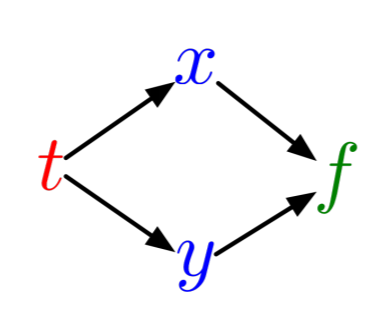
i.e. $t$ directly determines $x$ and $y$ which then determines $f$. To calculate Assume you've already evaluated $f(t)$. If this has been done, then you've already had to calculate $x$ and $y$. Thus given the function $f$, we can now calculate $\frac{df}{dx}$ and $\frac{df}{dy}$, and then calculate $\frac{dx}{dt}$ and $\frac{dy}{dt}$.
Now let's put another layer in the computation. Let's make $f(x(v(t),w(t)),y(v(t),w(t))$. We can write out the full expression for the derivative. Notice that even with this additional layer, the statement we wrote above still holds:
\[ \frac{df}{dt} = \frac{df}{dx}\frac{dx}{dt} + \frac{df}{dy}\frac{dy}{dt} \]
So given an evaluation of $f$, we can (still) directly calculate $\frac{df}{dx}$ and $\frac{df}{dy}$. But now, to calculate $\frac{dx}{dt}$ and $\frac{dy}{dt}$, we do the next step of the chain rule:
\[ \frac{dx}{dt} = \frac{dx}{dv}\frac{dv}{dt} + \frac{dx}{dw}\frac{dw}{dt} \]
and similar for $y$. So plug it all in, and you see that our equations will grow wild if we actually try to plug it in! But it's clear that, to calculate $\frac{df}{dt}$, we can first calculate $\frac{df}{dx}$, and then multiply that to $\frac{dx}{dt}$. If we had more layers, we could calculate the sensitivity (the derivative) of the output to the last layer, then and then the sensitivity to the second layer back is the sensitivity of the last layer multiplied to that, and the third layer back has the sensitivity of the second layer multiplied to it!
Logistic Regression Example
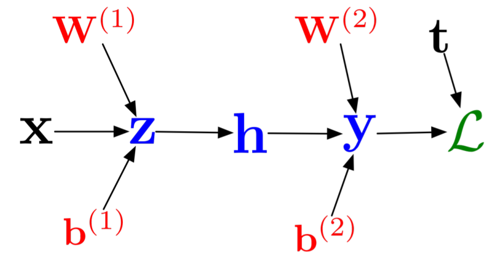
To better see this structure, let's write out a simple example. Let our forward pass through our function be:
\[ \begin{align} z &= wx + b\\ y &= \sigma(z)\\ \mathcal{L} &= \frac{1}{2}(y-t)^2\\ \mathcal{R} &= \frac{1}{2}w^2\\ \mathcal{L}_{reg} &= \mathcal{L} + \lambda \mathcal{R}\end{align} \]
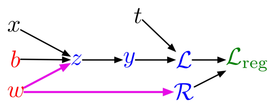
The formulation of the program here is called a Wengert list, tape, or graph. In this, $x$ and $t$ are inputs, $b$ and $W$ are parameters, $z$, $y$, $\mathcal{L}$, and $\mathcal{R}$ are intermediates, and $\mathcal{L}_{reg}$ is our output.
This is a simple univariate logistic regression model. To do logistic regression, we wish to find the parameters $w$ and $b$ which minimize the distance of $\mathcal{L}_{reg}$ from a desired output, which is done by computing derivatives.
Let's calculate the derivatives with respect to each quantity in reverse order. If our program is $f(x) = \mathcal{L}_{reg}$, then we have that
\[ \frac{df}{d\mathcal{L}_{reg}} = 1 \]
as the derivatives of the last layer. To computerize our notation, let's write
\[ \overline{\mathcal{L}_{reg}} = \frac{df}{d\mathcal{L}_{reg}} \]
for our computed values. For the derivatives of the second to last layer, we have that:
\[ \begin{align} \overline{\mathcal{R}} &= \frac{df}{d\mathcal{L}_{reg}} \frac{d\mathcal{L}_{reg}}{d\mathcal{R}}\\ &= \overline{\mathcal{L}_{reg}} \lambda \end{align} \]
\[ \begin{align} \overline{\mathcal{L}} &= \frac{df}{d\mathcal{L}_{reg}} \frac{d\mathcal{L}_{reg}}{d\mathcal{L}}\\ &= \overline{\mathcal{L}_{reg}} \end{align} \]
This was our observation from before that the derivative of the second layer is the partial derivative of the current values times the sensitivity of the final layer. And then we keep multiplying, so now for our next layer we have that:
\[ \begin{align} \overline{y} &= \overline{\mathcal{L}} \frac{d\mathcal{L}}{dy}\\ &= \overline{\mathcal{L}} (y-t) \end{align} \]
And notice that the chain rule holds since $\overline{\mathcal{L}}$ implicitly already has the multiplication by $\overline{\mathcal{L}_{reg}}$ inside of it. Then the next layer is:
\[ \begin{align} \frac{df}{z} &= \overline{y} \frac{dy}{dz}\\ &= \overline{y} \sigma^\prime(z) \end{align} \]
Then the next layer. Notice that here, by the chain rule on $w$ we have that:
\[ \begin{align} \overline{w} &= \overline{z} \frac{\partial z}{\partial w} + \overline{\mathcal{R}} \frac{d \mathcal{R}}{dw}\\ &= \overline{z} x + \overline{\mathcal{R}} w\end{align} \]
\[ \begin{align} \overline{b} &= \overline{z} \frac{\partial z}{\partial b}\\ &= \overline{z} \end{align} \]
This completely calculates all derivatives. In conclusion, the rule is:
You sum terms from each outward arrow
Each arrow has the derivative term of the end times the partial of the current term.
Recurse backwards to build simple linear combination expressions.
You can thus think of the relations as a message passing relation in reverse to the forward pass:
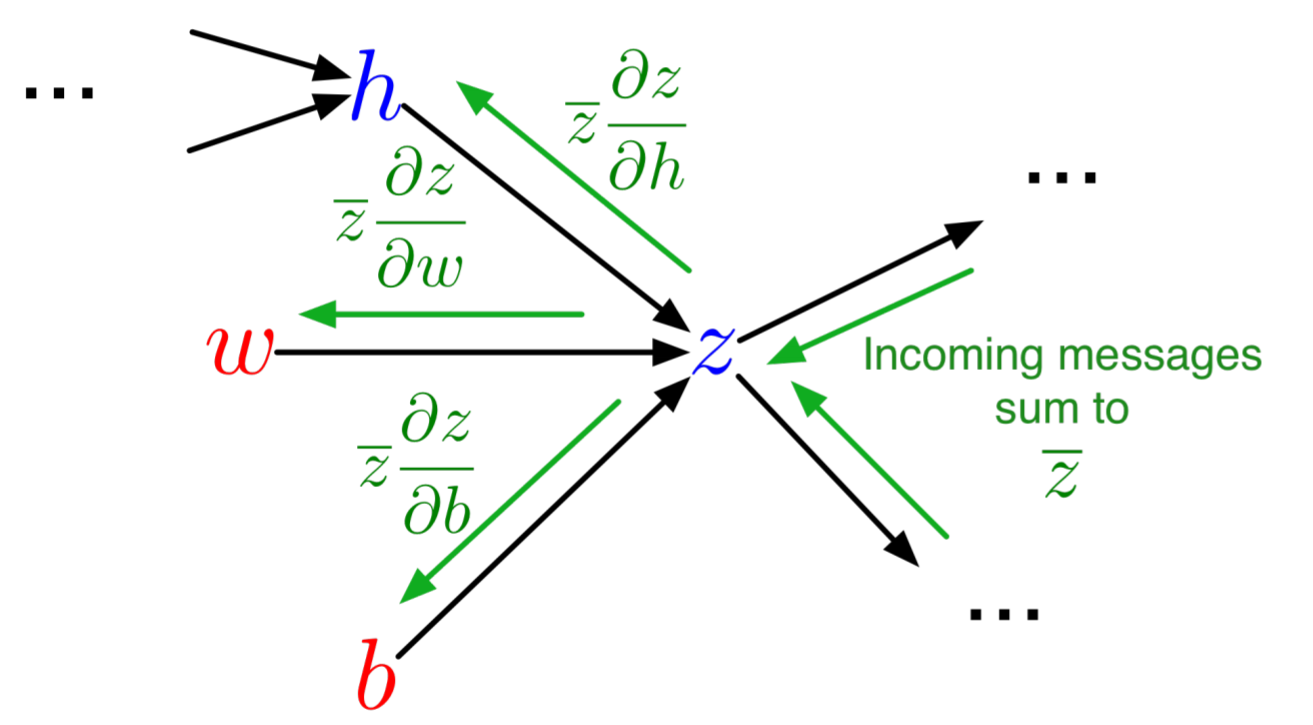
Note that the reverse-pass has the values of the forward pass, like $x$ and $t$, embedded within it.
Backpropagation of a Neural Network
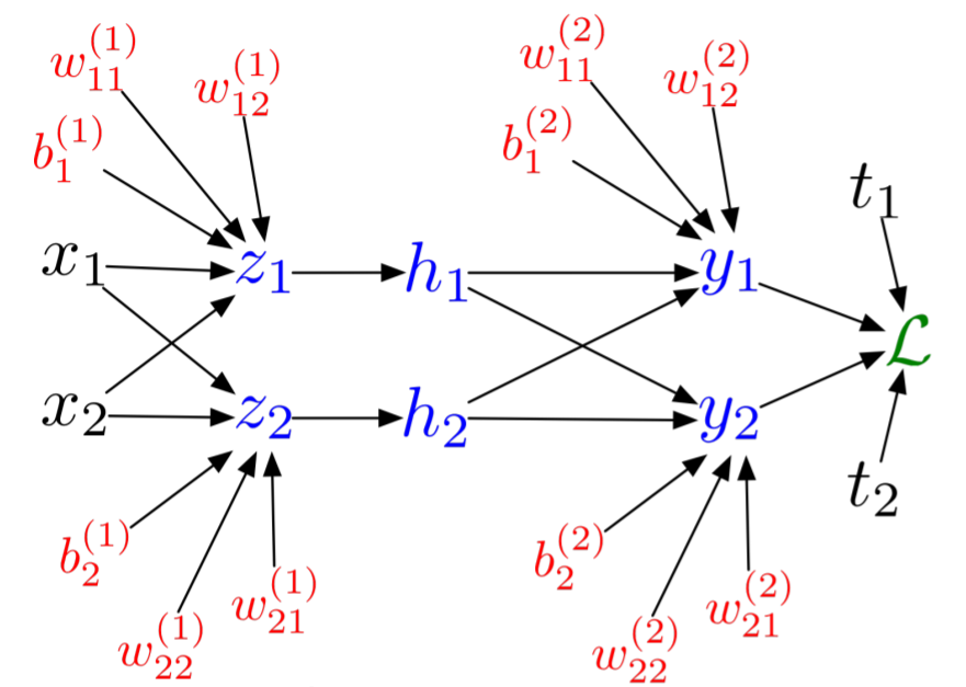
Now let's look at backpropagation of a deep neural network. Before getting to it in the linear algebraic sense, let's write everything in terms of scalars. This means we can write a simple neural network as:
\[ \begin{align} z_i &= \sum_j W_{ij}^1 x_j + b_i^1\\ h_i &= \sigma(z_i)\\ y_i &= \sum_j W_{ij}^2 h_j + b_i^2\\ \mathcal{L} &= \frac{1}{2} \sum_k \left(y_k - t_k \right)^2 \end{align} \]
where I have chosen the L2 loss function. This is visualized by the computational graph:
Then we can do the same process as before to get:
\[ \begin{align} \overline{\mathcal{L}} &= 1\\ \overline{y_i} &= \overline{\mathcal{L}} (y_i - t_i)\\ \overline{w_{ij}^2} &= \overline{y_i} h_j\\ \overline{b_i^2} &= \overline{y_i}\\ \overline{h_i} &= \sum_k (\overline{y_k}w_{ki}^2)\\ \overline{z_i} &= \overline{h_i}\sigma^\prime(z_i)\\ \overline{w_{ij}^1} &= \overline{z_i} x_j\\ \overline{b_i^1} &= \overline{z_i}\end{align} \]
just by examining the computation graph. Now let's write this in linear algebraic form.
The forward pass for this simple neural network was:
\[ \begin{align} z &= W_1 x + b_1\\ h &= \sigma(z)\\ y &= W_2 h + b_2\\ \mathcal{L} = \frac{1}{2} \Vert y-t \Vert_2^2 \end{align} \]
If we carefully decode our scalar expression, we see that we get the following:
\[ \begin{align} \overline{\mathcal{L}} &= 1\\ \overline{y} &= \overline{\mathcal{L}}(y-t)\\ \overline{W_2} &= \overline{y}h^{T}\\ \overline{b_2} &= \overline{y}\\ \overline{h} &= W_2^T \overline{y}\\ \overline{z} &= \overline{h} .* \sigma^\prime(z)\\ \overline{W_1} &= \overline{z} x^T\\ \overline{b_1} &= \overline{z} \end{align} \]
We can thus decode the rules as:
Multiplying by the matrix going forwards means multiplying by the transpose going backwards. A term on the left stays on the left, and a term on the right stays on the right.
Element-wise operations give element-wise multiplication
Notice that the summation is then easily encoded into this rule by the transpose operation.
We can write it in the general DNN form of:
\[ r_i = W_i v_{i} + b_i \]
\[ v_{i+1} = \sigma_i.(r_i) \]
\[ v_1 = x \]
\[ \mathcal{L} = \frac{1}{2} \Vert v_{n} - t \Vert_2 \]
\[ \begin{align} \overline{\mathcal{L}} &= 1\\ \overline{v_n} &= \overline{\mathcal{L}}(y-t)\\ \overline{r_i} &= \overline{v_i} .* \sigma_i^\prime (r_i)\\ \overline{W_i} &= \overline{v_i}r_{i-1}^{T}\\ \overline{b_i} &= \overline{v_i}\\ \overline{v_{i-1}} &= W_{i}^{T} \overline{v_i} \end{align} \]
Reverse-Mode Automatic Differentiation and vjps
Backpropagation of a neural network is thus a different way of accumulating derivatives. If $f$ is a composition of $L$ functions:
\[ f = f^L \circ f^{L-1} \circ \ldots \circ f^1 \]
Then the Jacobian matrix satisfies:
\[ J = J_L J_{L-1} \ldots J_1 \]
A program is essentially a nice way of writing a function in composition form. Forward-mode automatic differentiation worked by propagating forward the actions of the Jacobians at every step of the program:
\[ Jv = J_L (J_{L-1} (\ldots (J_1 v) \ldots )) \]
effectively calculating the Jacobian of the program by multiplying by the Jacobians from left to right at each step of the way. This means doing primitive $Jv$ calculations on each underlying problem, and pushing that calculation through.
But what about reverse accumulation? This can be isolated to the simple expression graph:
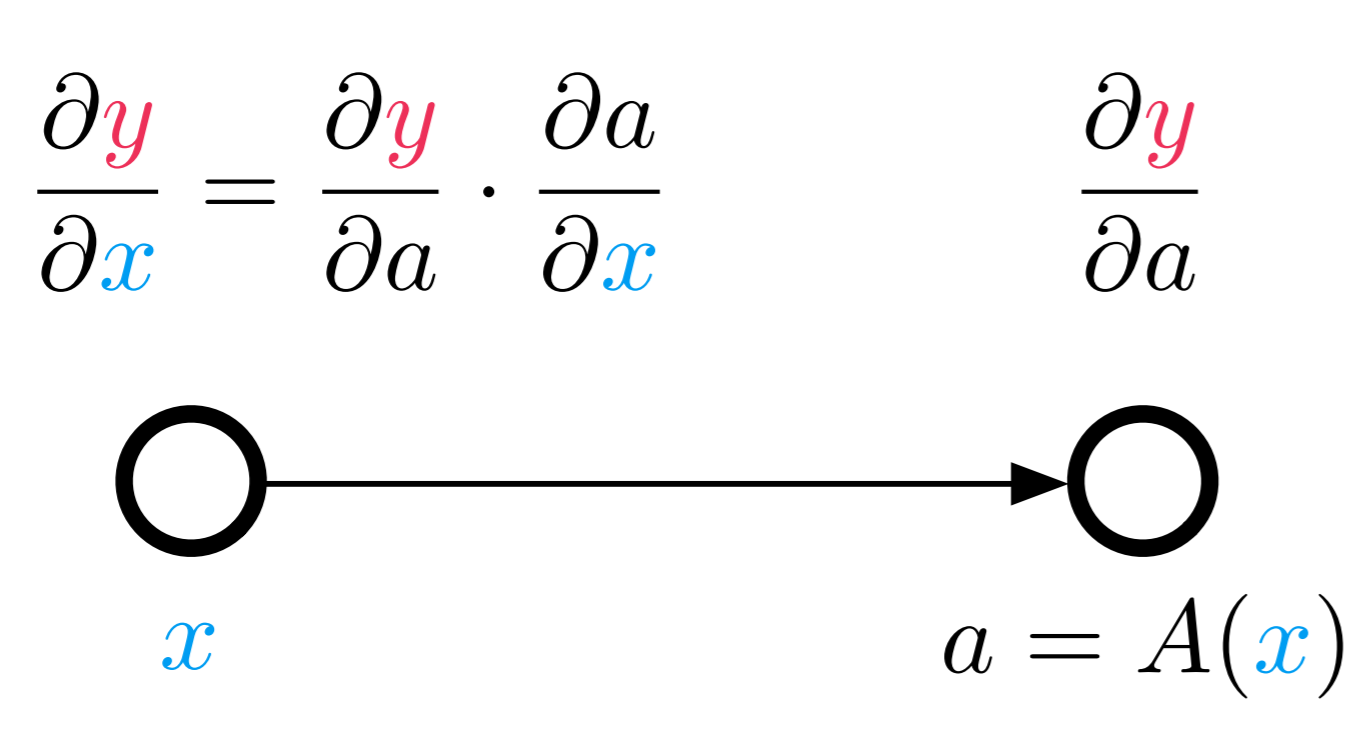
In backpropagation, we just showed that when doing reverse accumulation, the rule is that multiplication forwards is multiplication by the transpose backwards. So if the forward way to compute the Jacobian in reverse is to replace the matrix by its transpose:
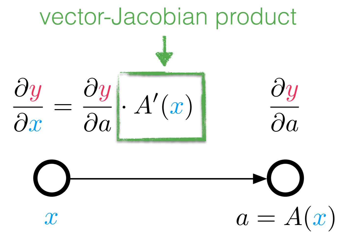
We can either look at it as $J^T v$, or by transposing the equation $v^T J$. It's right there that we have a vector-transpose Jacobian product, or a vjp.
We can thus think of this as a different direction for the Jacobian accumulation. Reverse-mode automatic differentiation moves backwards through our composed Jacobian. For a value $v$ at the end, we can push it backwards:
\[ v^T J = (\ldots ((v^T J_L) J_{L-1}) \ldots ) J_1 \]
doing a vjp at every step of the way, which is simply doing reverse-mode AD of that function (and if it's linear, then simply doing the matrix multiplication). Thus reverse-mode AD is just a grouping of vjps into a single larger expression, instead of linearizing every single step.
Primitives of Reverse Mode
For forward-mode AD, we saw that we could define primitives in order to accelerate the calculation. For example, knowing that
\[ exp(x+\epsilon) = exp(x) + exp(x)\epsilon \]
allows the program to skip autodifferentiating through the code for exp. This was simple with forward-mode since we could represent the operation on a Dual number. What's the equivalent for reverse-mode AD? The answer is the pullback function. If $y = [y_1,y_2,\ldots] = f(x_1,x_2, \ldots)$, then $[\overline{x_1},\overline{x_2},\ldots]=\mathcal{B}_f^x(\overline{y})$ is the pullback of $f$ at the point $x$, defined for a scalar loss function $L(y)$ as:
\[ \overline{x_i} = \frac{\partial L}{\partial x_i} = \sum_j \frac{\partial L}{\partial y_j} \frac{\partial y_j}{\partial x_i} \]
Using the notation from earlier, $\overline{y} = \frac{\partial L}{\partial y}$ is the derivative of some intermediate w.r.t. the cost function, and thus
\[ \overline{x_i} = \sum_j \overline{y_j} \frac{\partial y_j}{\partial x_i} = (\mathcal{B}_f^x(\overline{y}))_i \]
Note that $\mathcal{B}_f^x(\overline{y})$ is a function of $x$ because the reverse pass that is use embeds values from the forward pass, and the values from the forward pass to use are those calculated during the evaluation of $f(x)$.
By the chain rule, if we don't have a primitive defined for $y_i(x)$, we can compute that by $\mathcal{B}_{y_i}(\overline{y})$, and recursively apply this process until we hit rules that we know. The rules to start with are the scalar derivative rules with follow quite simply, and the multivariate rules which we derived above. For example, if $y=f(x)=Ax$, then
\[ \mathcal{B}_{f}^x(\overline{y}) = \overline{y}^T A \]
which is simply saying that the Jacobian of $f$ at $x$ is $A$, and so the vjp is to multiply the vector transpose by $A$.
Likewise, for element-wise operations, the Jacobian is diagonal, and thus the vjp is multiplying once again by a diagonal matrix against the derivative, deriving the same pullback as we had for backpropagation in a neural network. This then is a quicker encoding and derivation of backpropagation.
Multivariate Derivatives from Reverse Mode
Since the primitive of reverse mode is the vjp, we can understand its behavior by looking at a large primitive. In our simplest case, the function $f(x)=Ax$ outputs a vector value, which we apply our loss function $L(y) = \Vert y-t \Vert_2$ to get a scalar. Thus we seed the scalar output $v=1$, and in the first step backwards we have a vector to scalar function, so the first pullback transforms from $1$ to the vector $v_2 = 2|y-t|$. Then we take that vector and multiply it like $v_2^T A$ to get the derivatives w.r.t. $x$.
Now let $L(y)$ be a vector function, i.e. we output a vector instead of a scalar from our loss function. Then $v$ is the seed to this process. Let's assume that $v = e_i$, one of the basis vectors. Then
\[ v_i^T J = e_i^T J \]
pulls computes a row of the Jacobian. There, if we had a vector function $y=f(x)$, the pullback $\mathcal{B}_f^x(e_i)$ is the row of the Jacobian $f'(x)$. Concatenating these is thus a way to build a full Jacobian. The gradient is thus a special case where $y$ is scalar, and thus the resulting Jacobian is just a single row, and therefore we set the seed equal to $1$ to compute the unscaled gradient.
Multi-Seeding
Similarly to forward-mode having a dual number with multiple simultaneous derivatives through partials $d = x + v_1 \epsilon_1 + \ldots + v_m \epsilon_m$, one can see that multi-seeding is an option in reverse-mode AD by, instead of pulling back a matrix instead of a row vector, where each row is a direction. Thus the matrix $A = [v_1 v_2 \ldots v_n]^T$ evaluated as $\mathcal{B}_f^x(A)$ is the equivalent operation to the forward-mode $f(d)$ for generalized multivariate multiseeded reverse-mode automatic differentiation. One should take care to recognize the Jacobian as a generalized linear operator in this case and ensure that the shapes in the program correctly handle this storage of the reverse seed. When linear, this will automatically make use of BLAS3 operations, making it an efficient form for neural networks.
Sparse Reverse Mode AD
Since the Jacobian is built row-by-row with reverse mode AD, the sparse differentiation discussion from forward-mode AD applies similarly but to the transpose. Therefore, in order to perform sparse reverse mode automatic differentiation, one would build up a connectivity graph of the columns, and perform a coloring algorithm on this graph. The seeds of the reverse call, $v_i$, would then be the color vectors, which would compute compressed rows, that are then decompressed similarly to the forward-mode case.
Forward Mode vs Reverse Mode
Notice that a pullback of a single scalar gives the gradient of a function, while the pushforward using forward-mode of a dual gives a directional derivative. Forward mode computes columns of a Jacobian, while reverse mode computes gradients (rows of a Jacobian). Therefore, the relative efficiency of the two approaches is based on the size of the Jacobian. If $f:\mathbb{R}^n \rightarrow \mathbb{R}^m$, then the Jacobian is of size $m \times n$. If $m$ is much smaller than $n$, then computing by each row will be faster, and thus use reverse mode. In the case of a gradient, $m=1$ while $n$ can be large, leading to this phenomena. Likewise, if $n$ is much smaller than $m$, then computing by each column will be faster. We will see shortly the reverse mode AD has a high overhead with respect to forward mode, and thus if the values are relatively equal (or $n$ and $m$ are small), forward mode is more efficient.
However, since optimization needs gradients, reverse-mode definitely has a place in the standard toolchain which is why backpropagation is so central to machine learning.
Side Note on Mixed Mode
Interestingly, one can find cases where mixing the forward and reverse mode results would give an asymptotically better result. For example, if a Jacobian was non-zero in only the first 3 rows and first 3 columns, then sparse forward mode would still require N partials and reverse mode would require M seeds. However, one forward mode call of 3 partials and one reverse mode call of 3 seeds would calculate all three rows and columns with $\mathcal{O}(1)$ work, as opposed to $\mathcal{O}(N)$ or $\mathcal{O}(M)$. Exactly how to make use of this insight in an automated manner is an open research question.
Forward-Over-Reverse and Hessian-Free Products
Using this knowledge, we can also develop quick ways for computing the Hessian. Recall from earlier in the discussion that Hessians are the Jacobian of the gradient. So let's say for a scalar function $f$ we want to compute the Hessian. To compute the gradient, we use the reverse-mode AD pullback $\nabla f(x) = \mathcal{B}_f^x(1)$. Recall that the pullback is a function of $x$ since that is the value at which the values from the forward pass are taken. Then since the Jacobian of the gradient vector is $n \times n$ (as many terms in the gradient as there are inputs!), it holds that we want to use forward-mode AD for this Jacobian. Therefore, using the dual number $x = x_0 + e_1 \epsilon_1 + \ldots + e_n \epsilon_n$ the reverse mode gradient function computes the full Hessian in one forward pass. What this amounts to is pushing forward the dual number forward sensitivities when building the pullback, and then when doing the pullback the dual portions, will be holding vectors for the columns of the Hessian.
Similarly, Hessian-vector products without computing the Hessian can be computed using the Jacobian-vector product trick on the function defined by the gradient. Here, $Hv$ is equivalent to the dual part of
\[ \nabla f(x+v\epsilon) = \mathcal{B}_f^{x+v\epsilon}(1) \]
This means that our Newton method for optimization:
\[ p_{i+1} = p_i - H(p_i)^{-1} \frac{dC(p_i)}{dp} \]
can be treated similarly to that for the nonlinear solving problem, where the linear system can be solved using Hessian-free vector products to build a Krylov subspace, giving rise to the Hessian-free Newton Krylov method for optimization.
References
We thank Roger Grosse's lecture notes for the amazing tikz graphs.