Differentiable Programming and Neural Differential Equations

Chris Rackauckas

November 20th, 2020

Youtube Video Link

Our last discussion focused on how, at a high mathematical level, one could in theory build programs which compute gradients in a fast manner by looking at the computational graph and performing reverse-mode automatic differentiation. Within the context of parameter identification, we saw many advantages to this approach because it did not scale multiplicatively in the number of parameters, and thus it is an efficient way to calculate Jacobians of objects where there are less rows than columns (think of the gradient as 1 row).

More precisely, this is seen to be more about sparsity patterns, with reverse-mode as being more efficient if there are "enough" less row seeds required than column partials (with mixed mode approaches sometimes being much better). However, to make reverse-mode AD realistically usable inside of a programming language instead of a compute graph, we need to do three things:

1. We need to have a way of implementing reverse-mode AD on a language.

2. We need a systematic way to derive "adjoint" relationships (pullbacks).

3. We need to see if there are better ways to fit parameters to data, rather than performing reverse-mode AD through entire programs!

Implementation of Reverse-Mode AD

Forward-mode AD was implementable through operator overloading and dual number arithmetic. However, reverse-mode AD requires reversing a program through its computational structure, which is a much more difficult operation. This begs the question, how does one actually build a reverse-mode AD implementation?

Static Graph AD

The most obvious solution is to use a static compute graph since how we defined our differentiation structure was on a compute graph. Tensorflow is a modern example of this approach, where a user must define variables and operations in a graph language (that's embedded into Python, R, Julia, etc.), and then execution on the graph is easy to differentiate. This has the advantage of being a simplified and controlled form, which means that not only differentiation transformations are possible, but also things like automatic parallelization. However, many see directly writing a (static) computation graph as a barrier for practical use since it requires completely rewriting all existing programs to this structure.

Tracing-Based AD and Wengert Lists

Recall that an alternative formulation of reverse-mode AD for composed functions

\[ f = f^L \circ f^{L-1} \circ \ldots \circ f^1 \]

is through pullbacks on the Jacobians:

\[ v^T J = (\ldots ((v^T J_L) J_{L-1}) \ldots ) J_1 \]

Therefore, if one can transform the program structure into a list of composed functions, then reverse-mode AD is the successive application of pullbacks going in the reverse direction:

\[ \mathcal{B}_{f}^{x}(A)=\mathcal{B}_{f^{1}}^{x}\left(\ldots\left(\mathcal{\mathcal{B}}_{f^{L-1}}^{f^{L-2}(f^{L-3}(\ldots f^{1}(x)\ldots))}\left(\mathcal{B}_{f^{L}}^{f^{L-1}(f^{L-2}(\ldots f^{1}(x)\ldots))}(A)\right)\right)\ldots\right) \]

Recall that the pullback $\mathcal{B}_f^x(\overline{y})$ requires knowing:

1. The operation being performed

2. The value $x$ of the forward pass

The idea is to then build a Wengert list that is from exactly the forward pass of a specific $x$, also known as a trace, and thus giving rise to tracing-based reverse-mode AD. This is the basis of many reverse-mode implementations, such as Julia's Tracker.jl (an old AD system used in ML), ReverseDiff.jl, PyTorch, Tensorflow Eager, Autograd, and Autograd.jl. It is widely adopted due to its simplicity in implementation.

Inspecting Tracker.jl

Tracker.jl is a very simple implementation to inspect. The definition of its number and array types are as follows:

struct Call{F,As<:Tuple}
  func::F
  args::As
end

mutable struct Tracked{T}
  ref::UInt32
  f::Call
  isleaf::Bool
  grad::T
  Tracked{T}(f::Call) where T = new(0, f, false)
  Tracked{T}(f::Call, grad::T) where T = new(0, f, false, grad)
  Tracked{T}(f::Call{Nothing}, grad::T) where T = new(0, f, true, grad)
end

mutable struct TrackedReal{T<:Real} <: Real
  data::T
  tracker::Tracked{T}
end

struct TrackedArray{T,N,A<:AbstractArray{T,N}} <: AbstractArray{T,N}
  tracker::Tracked{A}
  data::A
  grad::A
  TrackedArray{T,N,A}(t::Tracked{A}, data::A) where {T,N,A} = new(t, data)
  TrackedArray{T,N,A}(t::Tracked{A}, data::A, grad::A) where {T,N,A} = new(t, data, grad)
end

As expected, it replaces every single number and array with a value that will store not just perform the operation, but also build up a list of operations along with the values at every stage. Then pullback rules are implemented for primitives via the @grad macro. For example, the pullback for the dot product is implemented as:

@grad dot(xs, ys) = dot(data(xs), data(ys)), Δ -> (Δ .* ys, Δ .* xs)

This is read as: the value going forward is computed by using the Julia dot function on the arrays, and the pullback embeds the backs of the forward pass and uses Δ .* ys as the derivative with respect to x, and Δ .* xs as the derivative with respect to y. This element-wise nature makes sense given the diagonal-ness of the Jacobian.

Note that this also allows utilizing intermediates of the forward pass within the reverse pass. This is seen in the definition of the pullback of meanpool:

@grad function meanpool(x, pdims::PoolDims; kw...)
  y = meanpool(data(x), pdims; kw...)
  y, Δ -> (nobacksies(:meanpool, NNlib.∇meanpool(data.((Δ, y, x))..., pdims; kw...)), nothing)
end

where the derivative makes use of not only x, but also y so that the meanpool does not need to be re-calculated.

Using this style, Tracker.jl moves forward, building up the value and closures for the backpass and then recursively pulls back the input Δ to receive the derivative.

Source-to-Source AD

Given our previous discussions on performance, you should be horrified with how this approach handles scalar values. Each TrackedReal holds as Tracked{T} which holds a Call, not a Call{F,As<:Tuple}, and thus it's not strictly typed. Because it's not strictly typed, this implies that every single operation is going to cause heap allocations. If you measure this in PyTorch, TensorFlow Eager, Tracker, etc. you get around 500ns-2ms of overhead. This means that a 2ns + operation becomes... >500ns! Oh my!

This is not the only issue with tracing. Another issue is that the trace is value-dependent, meaning that every new value can build a new trace. Thus one cannot easily JIT compile a trace because it'll be different for every gradient calculation (you can compile it, but you better make sure the compile times are short!). Lastly, the Wengert list can be much larger than the code itself. For example, if you trace through a loop that is for i in 1:100000, then the trace will be huge, even if the function is relatively simple. This is directly demonstrated in the JAX "how it works" slide:

To avoid these issues, another version of reverse-mode automatic differentiation is source-to-source transformations. In order to do source code transformations, you need to know how to transform all language constructs via the reverse pass. This can be quite difficult (what is the "adjoint" of lock?), but when worked out this has a few benefits. First of all, you do not have to track values, meaning stack-allocated values can stay on the stack. Additionally, you can JIT compile one backpass because you have a single function used for all backpasses. Lastly, you don't need to unroll your loops! Instead, which each branch you'd need to insert some data structure to recall the values used from the forward pass (in order to invert in the right directions). However, that can be much more lightweight than a tracking pass.

This can be a difficult problem to do in a general programming language. In general it needs a strong programmatic representation to use as a compute graph. Google's engineers did an analysis when choosing Swift for TensorFlow and narrowed it down to either Swift or Julia due to their internal graph structures. Thus, it should be no surprise that the modern source-to-source AD systems are Zygote.jl for Julia, and Swift for TensorFlow in Swift. Additionally, older AD systems, like Tampenade, ADIFOR, and TAF, all for Fortran, were source-to-source AD systems.

Worked Example: Reverse-Mode AD on the Babylonian Square Root

To make the above discussion concrete, let's work through every AD strategy on a single function: the Babylonian method for computing $\sqrt{x}$.

function f(x)
    a = x
    for i in 1:300
        a = 0.5 * (a + x/a)
    end
    a
end

f (generic function with 3 methods)

This iteratively computes $\sqrt{x}$ via the recurrence $a_{n+1} = \frac{1}{2}(a_n + x/a_n)$. After 300 iterations starting from $a_0 = x$, the result converges to machine precision. Since $f(x) = \sqrt{x}$, the exact derivative is $f'(x) = \frac{1}{2\sqrt{x}}$.

Step 1: Lowering to a Three-Address Form

Before differentiating, we decompose each compound expression into elementary operations, each assigned to a temporary. This is the form that a compiler (or an AD system) actually sees:

function f_lowered(x)
    a = x
    for i in 1:300
        tmp1 = x / a
        tmp2 = a + tmp1
        a = 0.5 * tmp2
    end
    y = a
end

f_lowered (generic function with 1 method)

Each line is now a single primitive operation (/, +, *) whose derivative rule we know. This decomposition is the starting point for all AD strategies.

Step 2: Forward-Mode AD

In forward-mode AD, we propagate a tangent $\dot{v}$ alongside each value $v$. For each elementary operation, we apply the standard differentiation rule:

• \[ \text{tmp1} = x/a \implies \dot{\text{tmp1}} = (\dot{x} \cdot a - \dot{a} \cdot x)/a^2 \]

  (quotient rule)

• \[ \text{tmp2} = a + \text{tmp1} \implies \dot{\text{tmp2}} = \dot{a} + \dot{\text{tmp1}} \]

  (sum rule)

• \[ a = 0.5 \cdot \text{tmp2} \implies \dot{a} = 0.5 \cdot \dot{\text{tmp2}} \]

  (constant scaling)

Seeding with $\dot{x} = 1$ gives us $\dot{y} = f'(x)$ at the output:

function f_forward(x, dx)
    a, da = (x, dx)
    for i in 1:300
        tmp1, dtmp1 = (x / a, (dx * a - da * x) / a^2)
        tmp2, dtmp2 = (a + tmp1, da + dtmp1)
        a, da = (0.5 * tmp2, 0.5 * dtmp2)
    end
    y, dy = (a, da)
end

f_forward (generic function with 1 method)

f_forward(2.0, 1.0)  # (sqrt(2), 1/(2*sqrt(2)))

(1.414213562373095, 0.35355339059327373)

Forward-mode computes the derivative in a single forward sweep. Its cost scales with the number of input perturbation directions (one pass per seed), so it's efficient when there are few inputs and many outputs.

Step 3: Reverse-Mode AD — Dynamic Graph (Tape-Based)

This is the approach used by PyTorch, ReverseDiff.jl, and Tracker.jl. During the forward pass, we record a tape (Wengert list) of every operation performed, along with the node IDs of inputs and outputs. Each intermediate value gets a unique node ID. Then the reverse pass walks the tape backward, applying pullback rules and accumulating adjoints:

function apply_pullback(::typeof(identity), args, out, outbar)
    (outbar,)
end

function apply_pullback(::typeof(/), args, out, outbar)
    a, b = args
    (outbar / b, -outbar * a / b^2)
end

function apply_pullback(::typeof(+), args, out, outbar)
    (outbar, outbar)
end

function apply_pullback(::typeof(*), args, out, outbar)
    a, b = args
    (outbar * b, outbar * a)
end

apply_pullback (generic function with 4 methods)

The pullback of each primitive is just the transpose of its Jacobian applied to the incoming adjoint $\bar{v}$. For example, the pullback of $y = a/b$ gives $\bar{a} = \bar{y}/b$ and $\bar{b} = -\bar{y} \cdot a/b^2$, which are exactly the entries of $J^T \bar{y}$.

The forward pass builds the tape by assigning node IDs:

function f_reverse_dynamic_ad(x)
    node_id = 0
    next_id() = (node_id += 1; node_id)

    tape = []  # entries: (op, input_ids, output_id)
    is_constant = Set{Int}()

    x_id = next_id()

    a_id = next_id()
    push!(tape, (identity, (x_id,), a_id))

    const_05_id = next_id()
    push!(is_constant, const_05_id)

    for i in 1:300
        tmp1_id = next_id()
        push!(tape, (/, (x_id, a_id), tmp1_id))

        tmp2_id = next_id()
        push!(tape, (+, (a_id, tmp1_id), tmp2_id))

        a_id = next_id()
        push!(tape, (*, (const_05_id, tmp2_id), a_id))
    end

    y_id = a_id

    # Replay tape to get forward values
    node_vals = Dict{Int,Float64}()
    node_vals[x_id] = x
    node_vals[const_05_id] = 0.5

    for (op, in_ids, out_id) in tape
        args = ntuple(j -> node_vals[in_ids[j]], length(in_ids))
        node_vals[out_id] = op === identity ? args[1] : op(args...)
    end

    y = node_vals[y_id]

    function reversepass(ybar)
        adj = Dict{Int,Float64}()
        adj[y_id] = ybar

        for i in length(tape):-1:1
            op, in_ids, out_id = tape[i]
            outbar = get(adj, out_id, 0.0)
            args = ntuple(j -> node_vals[in_ids[j]], length(in_ids))
            bars = apply_pullback(op, args, node_vals[out_id], outbar)
            for (j, id) in enumerate(in_ids)
                if id ∉ is_constant
                    adj[id] = get(adj, id, 0.0) + bars[j]
                end
            end
        end
        get(adj, x_id, 0.0)
    end

    y, reversepass
end

f_reverse_dynamic_ad (generic function with 1 method)

y, pullback = f_reverse_dynamic_ad(2.0)
(y, pullback(1.0))

(1.414213562373095, 0.35355339059327373)

The reverse pass is completely generic — it dispatches on the recorded op via apply_pullback and accumulates adjoints by node ID. No knowledge of the specific program structure is needed. This generality is precisely why dynamic graph AD is so widely adopted: any program that can be traced produces a correct gradient.

The downside is visible in the implementation: we allocate a tape entry for every single scalar operation (900 entries for 300 loop iterations), and every intermediate value is stored in a Dict. For a 300-iteration loop, this is fine; for a deep neural network with millions of operations, this overhead becomes the bottleneck.

Step 4: Reverse-Mode AD — Memory-Based (Checkpointing All Values)

Instead of recording a generic tape, we can write a reverse pass that is specialized to the structure of our program. The key insight is that the reverse pass needs the values from the forward pass (to evaluate Jacobians), but not the tape machinery. So we simply store the intermediate values in an array:

function f_reverse_memory(x, da)
    # Forward pass: store all intermediate a values
    as = zeros(301)
    as[1] = x
    for i in 1:300
        tmp1 = x / as[i]
        tmp2 = as[i] + tmp1
        as[i+1] = 0.5 * tmp2
    end

    y = as[end]

    # Reverse pass
    abar = da
    xbar = 0.0

    for i in 300:-1:1
        # Reverse of: a[i+1] = 0.5 * tmp2
        tmp2bar = abar * 0.5

        # Reverse of: tmp2 = a[i] + tmp1
        tmp1bar = tmp2bar
        abar_from_add = tmp2bar

        # Reverse of: tmp1 = x / a[i]
        xbar += tmp1bar / as[i]
        abar_from_div = tmp1bar * (-x / as[i]^2)

        # Total adjoint for a[i]
        abar = abar_from_add + abar_from_div
    end

    # Reverse of initial: a = x
    xbar += abar

    y, xbar
end

f_reverse_memory (generic function with 1 method)

f_reverse_memory(2.0, 1.0)

(1.414213562373095, 0.35355339059327373)

The reverse pass is now just a loop — no dictionaries, no dispatch, no heap allocations per operation. Each line of the reverse loop is the adjoint of the corresponding line in the forward loop, read in reverse order:

Forward	Reverse
a[i+1] = 0.5 * tmp2	tmp2bar = abar * 0.5
tmp2 = a[i] + tmp1	abar += tmp2bar; tmp1bar = tmp2bar
tmp1 = x / a[i]	xbar += tmp1bar/a[i]; abar += -tmp1bar*x/a[i]^2

Note how xbar accumulates a contribution from every iteration, since x is used in tmp1 = x/a at every step. This is the "fan-out" rule: when a variable is used multiple times, its adjoint is the sum of all contributions.

The cost is $O(N)$ memory to store the as array, where $N$ is the number of iterations.

Step 5: Reverse-Mode AD — Memoryless (Enzyme/NiLang Style)

Source-to-source AD systems like Enzyme and NiLang can avoid storing intermediates entirely by inverting the forward computation. If we can reconstruct $a_{\text{old}}$ from $a_{\text{new}}$, we don't need the as array at all.

The forward step is $a_{\text{new}} = \frac{1}{2}(a_{\text{old}} + x/a_{\text{old}})$. Inverting: $\text{tmp2} = 2 a_{\text{new}}$, and $a_{\text{old}}$ satisfies $a_{\text{old}}^2 - \text{tmp2} \cdot a_{\text{old}} + x = 0$, giving $a_{\text{old}} = \frac{\text{tmp2} + \sqrt{\text{tmp2}^2 - 4x}}{2}$ (taking the larger root, since $a > \sqrt{x}$ throughout the iteration):

function f_reverse_memoryless(x, da)
    a = x
    for i in 1:300
        tmp1 = x / a
        tmp2 = a + tmp1
        a = 0.5 * tmp2
    end

    aout = a

    # Reverse pass: reconstruct intermediates by inverting each step
    abar = da
    xbar = 0.0

    for i in 300:-1:1
        # Invert: a_new = 0.5 * tmp2 => tmp2 = 2 * a
        tmp2 = 2 * a
        # Invert: a_old^2 - tmp2*a_old + x = 0 => take larger root
        a_old = (tmp2 + sqrt(abs(tmp2^2 - 4x))) / 2
        tmp1 = x / a_old

        tmp2bar = abar * 0.5
        tmp1bar = tmp2bar
        abar_from_add = tmp2bar

        xbar += tmp1bar / a_old
        abar_from_div = tmp1bar * (-x / a_old^2)

        abar = abar_from_add + abar_from_div
        a = a_old
    end

    xbar += abar

    aout, xbar
end

f_reverse_memoryless (generic function with 1 method)

f_reverse_memoryless(2.0, 1.0)

(1.414213562373095, 0.35355339059327234)

This uses $O(1)$ memory regardless of the number of iterations. The tradeoff is that the inversion (here, a quadratic formula) adds computation and can introduce small floating-point errors. For the Babylonian method specifically, the inversion is exact in exact arithmetic but introduces ~$10^{-15}$ error in floating point — acceptable for most applications.

Step 6: Dynamic Control Flow

What happens when the iteration count isn't fixed? Replace the for loop with a convergence-based while loop:

function f_while(x)
    a = x
    while abs(a - x/a) > 1e-14
        a = 0.5 * (a + x/a)
    end
    a
end

f_while (generic function with 1 method)

This changes nothing about the derivative rules — only about what the AD system must handle. For memory-based reverse AD, we store values as before but use a growable array:

function f_while_reverse_memory(x, da)
    as = [x]
    while abs(as[end] - x / as[end]) > 1e-14
        a_prev = as[end]
        tmp1 = x / a_prev
        tmp2 = a_prev + tmp1
        push!(as, 0.5 * tmp2)
    end

    y = as[end]
    abar = da
    xbar = 0.0

    for i in (length(as)):-1:2
        tmp2bar = abar * 0.5
        tmp1bar = tmp2bar
        abar_from_add = tmp2bar

        xbar += tmp1bar / as[i-1]
        abar_from_div = tmp1bar * (-x / as[i-1]^2)

        abar = abar_from_add + abar_from_div
    end

    xbar += abar
    y, xbar
end

f_while_reverse_memory (generic function with 1 method)

For the memoryless version, we just need to count iterations:

function f_while_reverse_memoryless(x, da)
    a = x
    iters = 0
    while abs(a - x/a) > 1e-14
        iters += 1
        tmp1 = x / a
        tmp2 = a + tmp1
        a = 0.5 * tmp2
    end

    aout = a
    abar = da
    xbar = 0.0

    for i in iters:-1:1
        tmp2 = 2 * a
        a_old = (tmp2 + sqrt(abs(tmp2^2 - 4x))) / 2
        tmp1 = x / a_old

        tmp2bar = abar * 0.5
        tmp1bar = tmp2bar
        abar_from_add = tmp2bar

        xbar += tmp1bar / a_old
        abar_from_div = tmp1bar * (-x / a_old^2)

        abar = abar_from_add + abar_from_div
        a = a_old
    end

    xbar += abar
    aout, xbar
end

f_while_reverse_memoryless (generic function with 1 method)

f_while_reverse_memory(2.0, 1.0)

(1.414213562373095, 0.35355339059327373)

f_while_reverse_memoryless(2.0, 1.0)

(1.414213562373095, 0.35355339059327473)

Dynamic control flow is where the tradeoffs between AD strategies become sharp:

• Tracing-based AD (PyTorch, JAX) unrolls the while loop into a flat trace. The trace length varies per input — you cannot JIT compile it once.

• Memory-based AD stores values as the loop runs. The memory cost is proportional to the (unknown in advance) iteration count.

• Memoryless/source-to-source AD (Enzyme) only needs to record the iteration count (a single integer), then inverts each step. This is why Enzyme can differentiate through complex loops and solvers with minimal overhead.

Summary: Comparing the Strategies

Let's verify all implementations against the exact derivative:

x = 2.0
exact = 1 / (2*sqrt(x))

_, d_fwd = f_forward(x, 1.0)
_, d_mem = f_reverse_memory(x, 1.0)
_, d_mless = f_reverse_memoryless(x, 1.0)
_, pb = f_reverse_dynamic_ad(x)
d_dyn = pb(1.0)
_, d_wmem = f_while_reverse_memory(x, 1.0)
_, d_wmless = f_while_reverse_memoryless(x, 1.0)

println("Exact derivative:        $exact")
println("Forward-mode:            $d_fwd    (err = $(abs(d_fwd - exact)))")
println("Reverse dynamic (tape):  $d_dyn    (err = $(abs(d_dyn - exact)))")
println("Reverse memory:          $d_mem    (err = $(abs(d_mem - exact)))")
println("Reverse memoryless:      $d_mless  (err = $(abs(d_mless - exact)))")
println("While + memory:          $d_wmem   (err = $(abs(d_wmem - exact)))")
println("While + memoryless:      $d_wmless (err = $(abs(d_wmless - exact)))")

Exact derivative:        0.35355339059327373
Forward-mode:            0.35355339059327373    (err = 0.0)
Reverse dynamic (tape):  0.35355339059327373    (err = 0.0)
Reverse memory:          0.35355339059327373    (err = 0.0)
Reverse memoryless:      0.35355339059327234  (err = 1.3877787807814457e-15
)
While + memory:          0.35355339059327373   (err = 0.0)
While + memoryless:      0.35355339059327473 (err = 9.992007221626409e-16)

Strategy	Memory	Tape overhead	Handles dynamic control flow	Examples
Forward-mode	$O(1)$	None	Yes (naturally)	ForwardDiff.jl, dual numbers
Reverse dynamic	$O(N)$	Dict + alloc	Yes (re-traces each call)	PyTorch, JAX, Tracker.jl, ReverseDiff.jl
Reverse memory	$O(N)$	None	Yes (growable arrays)	Checkpointing schemes
Reverse memoryless	$O(1)$	None	Yes (count only)	Enzyme, NiLang
Source-to-source	Varies	None	Yes (with analysis)	Zygote.jl, Enzyme, Tapenade

Derivation of Reverse Mode Rules: Adjoints and Implicit Function Theorem

Now this shows how reverse-mode AD generally works, and we can see from the general implementation that the key is to implement apply_pullback rules on specific primitive operations. This is just like the primitive rules for forward-mode AD, except now computing the vector-Jacobian product.

While this is easy to do for simple mathematical operations, you may be asking, if I have a complicated function, how do I derive the apply_pullback rules? It terns out that this intersects with an area of computational science known as adjoint methods. Adjoint methods are apply_pullback reverse-mode AD rules in disguise!

In order to require the least amount of work from our AD system, we need to be able to derive the adjoint rules at the highest level possible. Here are a few well-known cases to start understanding. These next examples are from Steven Johnson's resource.

Let's go through the full derivation of a few.

Adjoint of Linear Solve

Let's say we have the function $A(p)x=b(p)$, i.e. this is the function that is given by the linear solving process, and we want to calculate the gradients of a cost function $g(x,p)$. To evaluate the gradient directly, we'd calculate:

\[ \frac{dg}{dp} = g_p + g_x x_p \]

where $x_p$ is the derivative of each value of $x$ with respect to each parameter $p$, and thus it's an $M \times P$ matrix (a Jacobian). Since $g$ is a small cost function, $g_p$ and $g_x$ are easy to compute, but $x_p$ is given by:

\[ x_{p_i} = A^{-1}(b_{p_i}-A_{p_i}x) \]

and so this is $P$ $M \times M$ linear solves, which is expensive! However, if we multiply by

\[ \lambda^{T} = g_x A^{-1} \]

then we obtain

\[ \frac{dg}{dp}\vert_{f=0} = g_p - \lambda^T f_p = g_p - \lambda^T (A_p x - b_p) \]

which is an alternative formulation of the derivative at the solution value. However, in this case, there is no computational benefit to this reformulation.

Adjoint of Nonlinear Solve

Now let's look at some $f(x,p)=0$ nonlinear solving. Differentiating by $p$ gives us:

\[ f_x x_p + f_p = 0 \]

and thus $x_p = -f_x^{-1}f_p$. Therefore, using our cost function we write:

\[ \frac{dg}{dp} = g_p + g_x x_p = g_p - g_x \left(f_x^{-1} f_p \right) \]

or

\[ \frac{dg}{dp} = g_p - \left(g_x f_x^{-1} \right) f_p \]

Since $g_x$ is $1 \times M$, $f_x^{-1}$ is $M \times M$, and $f_p$ is $M \times P$, this grouping changes the problem and gets rid of the size $MP$ term.

As is normal with backpasses, we solve for $x$ through the forward pass however we like, and then for the backpass solve for

\[ f_x^T \lambda = g_x^T \]

to obtain

\[ \frac{dg}{dp}\vert_{f=0} = g_p - \lambda^T f_p \]

which does the calculation without ever building the size $M \times MP$ term.

Adjoint of Ordinary Differential Equations

We wish to solve for some cost function $G(u,p)$ evaluated throughout the differential equation, i.e.:

\[ G(u,p) = G(u(p)) = \int_{t_0}^T g(u(t,p))dt \]

To derive this adjoint, introduce the Lagrange multiplier $\lambda$ to form:

\[ I(p) = G(p) - \int_{t_0}^T \lambda^\ast (u^\prime - f(u,p,t))dt \]

Since $u^\prime = f(u,p,t)$, this is the mathematician's trick of adding zero, so then we have that

\[ \frac{dG}{dp} = \frac{dI}{dp} = \int_{t_0}^T (g_p + g_u s)dt - \int_{t_0}^T \lambda^\ast (s^\prime - f_u s - f_p)dt \]

for $s$ being the sensitivity, $s = \frac{du}{dp}$. After applying integration by parts to $\lambda^\ast s^\prime$, we get that:

\[ \int_{t_{0}}^{T}\lambda^{\ast}\left(s^{\prime}-f_{u}s-f_{p}\right)dt =\int_{t_{0}}^{T}\lambda^{\ast}s^{\prime}dt-\int_{t_{0}}^{T}\lambda^{\ast}\left(f_{u}s+f_{p}\right)dt \]

\[ =|\lambda^{\ast}(t)s(t)|_{t_{0}}^{T}-\int_{t_{0}}^{T}\lambda^{\ast\prime}sdt-\int_{t_{0}}^{T}\lambda^{\ast}\left(f_{u}s+f_{p}\right)dt \]

To see where we ended up, let's re-arrange the full expression now:

\[ \frac{dG}{dp} =\int_{t_{0}}^{T}(g_{p}+g_{u}s)dt+|\lambda^{\ast}(t)s(t)|_{t_{0}}^{T}-\int_{t_{0}}^{T}\lambda^{\ast\prime}sdt-\int_{t_{0}}^{T}\lambda^{\ast}\left(f_{u}s+f_{p}\right)dt \]

\[ =\int_{t_{0}}^{T}(g_{p}+\lambda^{\ast}f_{p})dt+|\lambda^{\ast}(t)s(t)|_{t_{0}}^{T}-\int_{t_{0}}^{T}\left(\lambda^{\ast\prime}+\lambda^\ast f_{u}-g_{u}\right)sdt \]

That was just a re-arrangement. Now, let's require that

\[ \lambda^\prime = -\frac{df}{du}^\ast \lambda + \left(\frac{dg}{du} \right)^\ast \]

\[ \lambda(T) = 0 \]

This means that one of the boundary terms of the integration by parts is zero, and also one of those integrals is perfectly zero. Thus, if $\lambda$ satisfies that equation, then we get:

\[ \frac{dG}{dp} = \lambda^\ast(t_0)\frac{du(t_0)}{dp} + \int_{t_0}^T \left(g_p + \lambda^\ast f_p \right)dt \]

which gives us our adjoint derivative relation.

If $G$ is discrete, then it can be represented via the Dirac delta:

\[ G(u,p) = \int_{t_0}^T \sum_{i=1}^N \Vert d_i - u(t_i,p)\Vert^2 \delta(t_i - t)dt \]

in which case

\[ g_u(t_i) = 2(d_i - u(t_i,p)) \]

at the data points $(t_i,d_i)$. Therefore, the derivatives of a cost function with respect to the parameters are obtained by solving for $\lambda^\ast$ using an ODE for $\lambda^T$ in reverse time, and then using that to calculate $\frac{dG}{dp}$. Note that $\frac{dG}{dp}$ can be calculated simultaneously by appending a single value to the reverse ODE, since we can simply define the new ODE term as $g_p + \lambda^\ast f_p$, which would then calculate the integral on the fly (ODE integration is just... integration!).

Complexities of Implementing ODE Adjoints

The image below explains the dilemma:

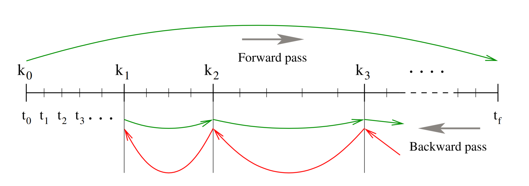
Essentially, the whole problem is that we need to solve the ODE

\[ \lambda^\prime = -\frac{df}{du}^\ast \lambda - \left(\frac{dg}{du} \right)^\ast \]

\[ \lambda(T) = 0 \]

in reverse, but $\frac{df}{du}$ is defined by $u(t)$ which is a value only computed in the forward pass (the forward pass is embedded within the backpass!). Thus we need to be able to retrieve the value of $u(t)$ to get the Jacobian on-demand. There are three ways in which this can be done:

1. If you solve the reverse ODE $u^\prime = f(u,p,t)$ backwards in time, mathematically it'll give equivalent values. Computation-wise, this means that you can append $u(t)$ to $\lambda(t)$ (to $\frac{dG}{dp}$) to calculate all terms at the same time with a single reverse pass ODE. However, numerically this is unstable and thus not always recommended (ODEs are reversible, but ODE solver methods are not necessarily going to generate the same exact values or trajectories in reverse!)

2. If you solve the forward ODE and receive a solution $u(t)$, you can interpolate it to retrieve the values at any time at which the reverse pass needs the $\frac{df}{du}$ Jacobian. This is fast but memory-intensive.

3. Every time you need a value $u(t)$ during the backpass, you re-solve the forward ODE to $u(t)$. This is expensive! Thus one can instead use checkpoints, i.e. save at a smaller number of time points during the forward pass, and use those as starting points for the $u(t)$ calculation.

Alternative strategies can be investigated, such as an interpolation that stores values in a compressed form.

The vjp and Neural Ordinary Differential Equations

It is here that we can note that, if $f$ is a function defined by a neural network, we arrive at the neural ordinary differential equation. This adjoint method is thus the backpropagation method for the neural ODE. However, the backpass

\[ \lambda^\prime = -\frac{df}{du}^\ast \lambda - \left(\frac{dg}{du} \right)^\ast \]

\[ \lambda(T) = 0 \]

can be improved by noticing $\lambda^\ast \frac{df}{du}$ is a vjp, and thus it can be calculated using $\mathcal{B}_f^{u(t)}(\lambda^\ast)$, i.e. reverse-mode AD on the function $f$. If $f$ is a neural network, this means that the reverse ODE is defined through successive backpropagation passes of that neural network. The result is a derivative of the cost function with respect to the parameters defining $f$ (either a model or a neural network), which can then be used to fit the data ("train").

Alternative "Training" Strategies

Those are the "brute force" training methods which simply use $u(t,p)$ evaluations to calculate the cost. However, it is worth noting that there are a few better strategies that one can employ in the case of dynamical models.

Multiple Shooting Techniques

Instead of shooting just from the beginning, one can instead shoot from multiple points in time:

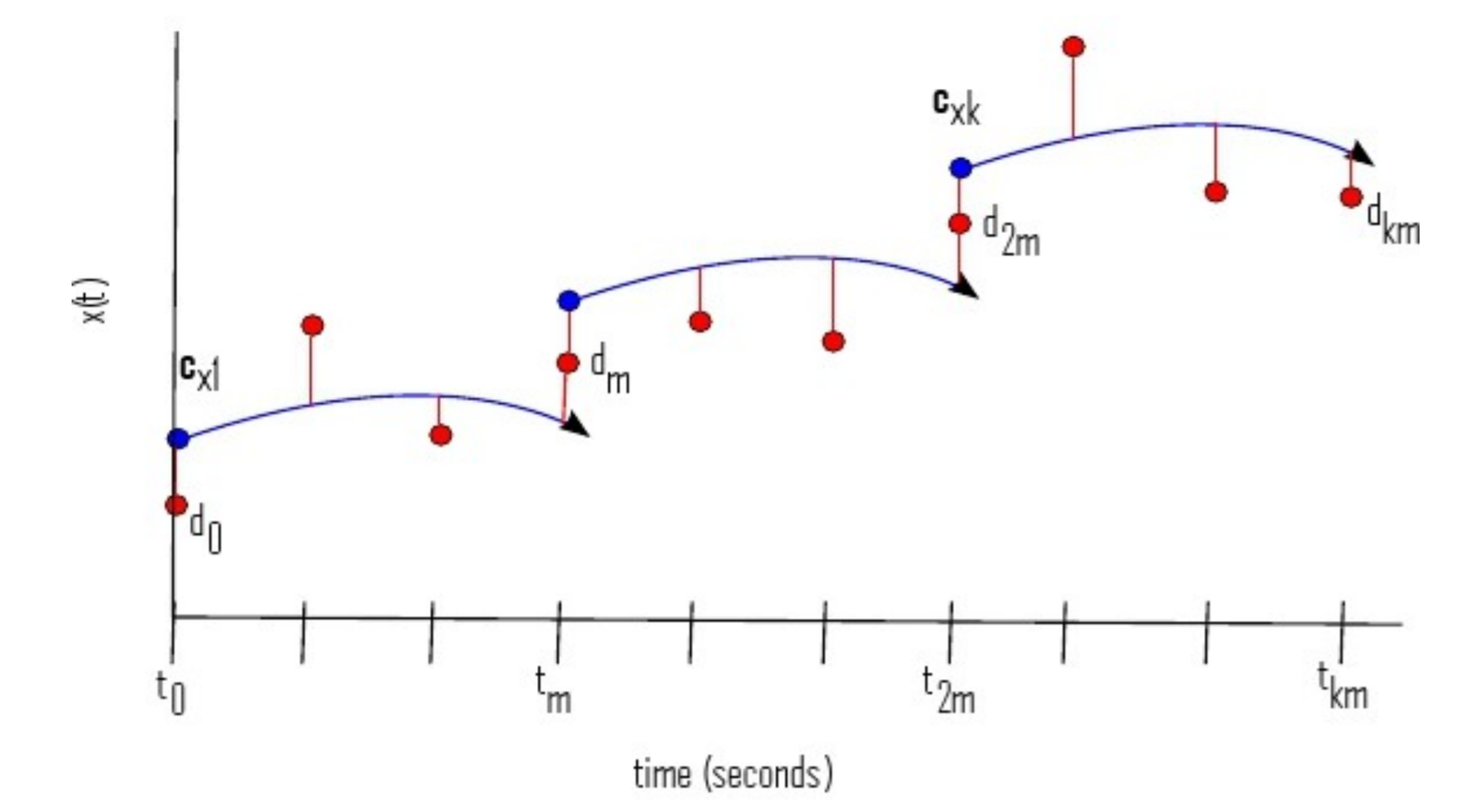
Of course, one won't know what the "initial condition in the future" is, but one can instead make that a parameter. By doing so, each interval can be solved independently, and one can then add to the cost function that the end of one interval must match up with the beginning of the other. This can make the integration more robust, since shooting with incorrect parameters over long time spans can give massive gradients which makes it hard to hone in on the correct values.

Collocation Methods

If the data is dense enough, one can fit a curve through the points, such as a spline:

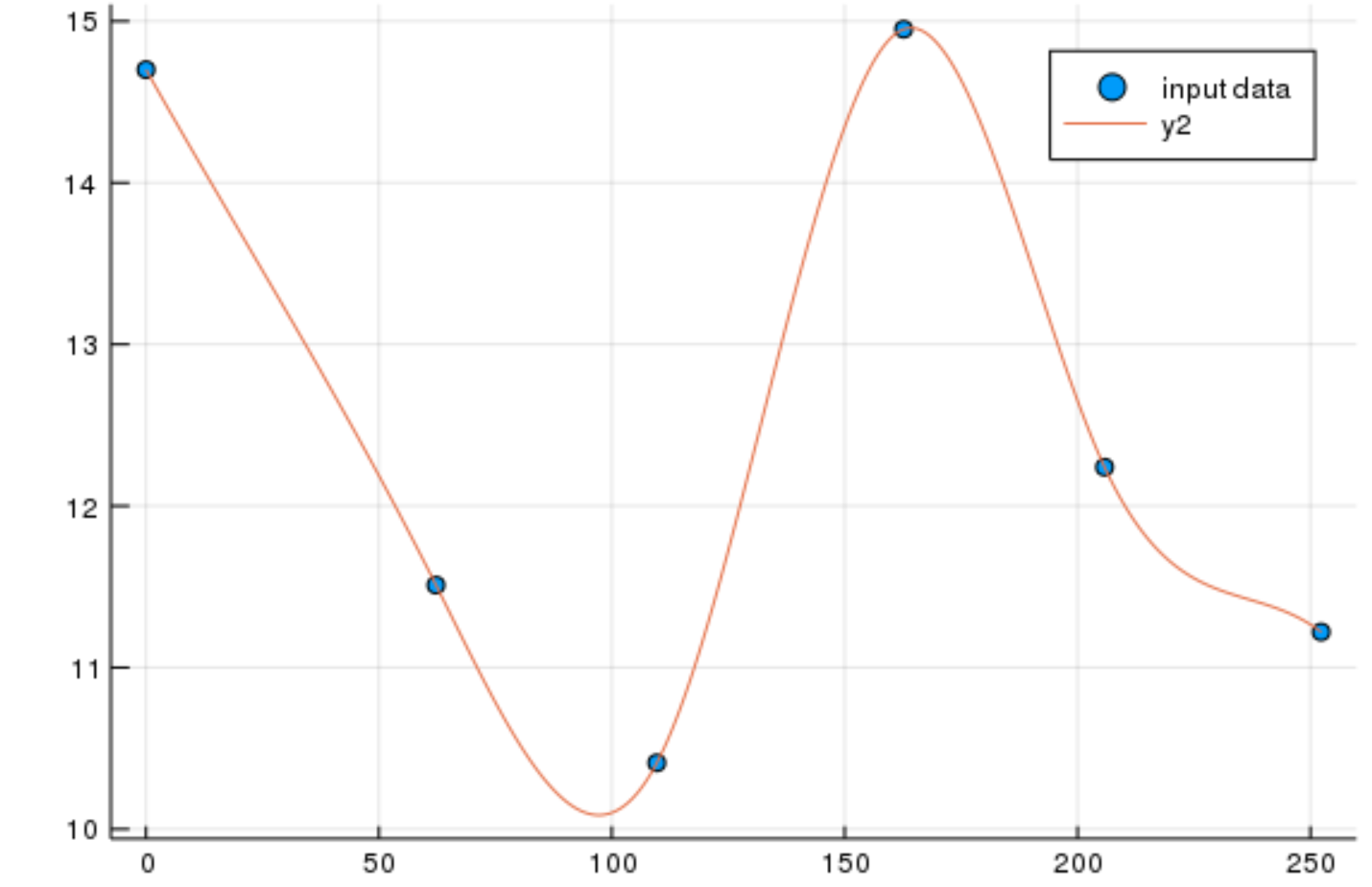
If that's the case, one can use the fit spline in order to estimate the derivative at each point. Since the ODE is defined as $u^\prime = f(u,p,t)$, one can then use the cost function

\[ C(p) = \sum_{i=1}^N \Vert\tilde{u}^{\prime}(t_i) - f(u(t_i),p,t)\Vert \]

where $\tilde{u}^{\prime}(t_i)$ is the estimated derivative at the time point $t_i$. Then one can fit the parameters to ensure this holds. This method can be extremely fast since the ODE doesn't ever have to be solved! However, note that this is not able to compensate for error accumulation, and thus early errors are not accounted for in the later parts of the data. This means that the integration won't necessarily match the data even if this fit is "good" if the data points are too far apart, a property that is not true with fitting. Thus, this is usually done as part of a two-stage method, where the starting stage uses collocation to get initial parameters which is then completed with a shooting method.