From Optimization to Probabilistic Programming
Chris Rackauckas
December 12th, 2020
Youtube Video
With a high degree of probability, all things are probabilistic. In all of the cases we have previously looked at (differential equations, neural networks, neural differential equations, physics-informed neural networks, etc.) we have incorporated data into our models using point estimates, i.e. getting "exact fits". However, data has noise and uncertainty. We want to extend our previous modeling approaches to include probabilistic estimates. This is known as probabilistic programming, or Bayesian estimation on general programming models. To approach this topic, we will first introduce the Bayesian way of thinking about variables as random variables, estimating probabilistic programs, and how efficient probabilistic programming frameworks incorporate differentiable programming.
Bayesian Modeling in a Nutshell
The idea of Bayesian modeling is to treat your variables as a random variable with respect to some distribution. As a starting point, think about the linear model
\[ f(x) = ax \]
The standard way to think of the linear model is that $a$ is a variable, and so you put a value $x$ in and compute $ax$. However, in the Bayesian sense, the value of $a$ can be a random variable. A random variable $Z$ is a variable which has probability of taking certain values from a probability distribution. If we say that $Z \sim f(y)$, then we are saying that the probability that $Z$ takes a value in the set $\Omega$ is:
\[ \int_\Omega f(y)dy \]
For example, if $Z$ is a scalar, then the probability that $Z \in [0,1]$ is:
\[ \int_0^1 f(y)dy \]
Discrete probability distributions can be handled by either using distribution quantities and measures in the integral, or by simply saying $f(y)$ is the probability that $Z = y$.
Given this representation of variables, $ax$ where $a$ follows a probability distribution induces a probability distribution on $f(x)$. To numerically acquire this distribution, one can use Monte Carlo sampling. This is simply the repeat process of:
Sample variables
Compute output
Repeatedly doing this produces samples of $f(x)$ from which a numerical representation of the distribution can be had. From there, going to a multivariable linear model like $f(x) = Ax$ is the same idea. Going to $f(x)$ where $f$ is an arbitrary program is still the same idea: sample every variable in the program, compute the output, and repeat for many samples. $f$ can be a neural network where all of the parameters are probabilistic, or it can be an ODE solver with probabilistic parameters.
Quick Example
Let's do a quick example with the Lotka-Volterra equations. Recall that this is the ordinary differential equation defined by the following system:
using OrdinaryDiffEq, Plots
function lotka_volterra(du,u,p,t)
  du[1] = p[1] * u[1] - p[2] * u[1]*u[2]
  du[2] = -p[3] * u[2] + p[4] * u[1]*u[2]
end
θ = [1.5,1.0,3.0,1.0]
u0 = [1.0;1.0]
tspan = (0.0,10.0)
prob1 = ODEProblem(lotka_volterra,u0,tspan,θ)
sol = solve(prob1,Tsit5())
plot(sol)

Now let's assume that the θ's are random. With Julia we can make variables into random variables by using Distributions.jl:
using Distributions
θ = [Uniform(0.5,1.5),Beta(5,1),Normal(3,0.5),Gamma(5,2)]
4-element Vector{Distribution{Univariate, Continuous}}:
 Uniform{Float64}(a=0.5, b=1.5)
 Beta{Float64}(α=5.0, β=1.0)
 Normal{Float64}(μ=3.0, σ=0.5)
 Gamma{Float64}(α=5.0, θ=2.0)
from which we can sample points and propagate through the solver:
_θ = rand.(θ)
prob1 = ODEProblem(lotka_volterra,u0,tspan,_θ)
sol = solve(prob1,Tsit5())
plot(sol)

and from which we can get an ensemble of solutions:
prob_func = function (prob,ctx)
  remake(prob,p=rand.(θ))
end
ensemble_prob = EnsembleProblem(ODEProblem(lotka_volterra,u0,tspan,θ),
                                prob_func = prob_func)
sol = solve(ensemble_prob,Tsit5(),EnsembleThreads(),trajectories=1000)

using DiffEqBase.EnsembleAnalysis
plot(EnsembleSummary(sol))

From just a few variables having probabilities, every variable has an induced probability: there is a probability distribution on the integrator states, the output at time t_i, etc.
Bayesian Estimation with Point Estimates: Bayes' Rule, Maximum Likelihood, and MAP
Recall from our previous studies that the difficult part of modeling is not necessarily the forward modeling approach, rather it's the incorporation of data or the estimation problem that is difficult. When your variables are now random distributions, how do you "fit" them?
The answer comes from Bayes' rule, which is the following. Assume you had a prior distribution $p(\theta)$ for the probability that $X$ is a given value $\theta$. Then the posterior probability distribution, $p(\theta|D)$, or the distribution which is updated to include data, is given by:
\[ p(\theta|D) = \frac{p(D|\theta)p(\theta)}{\int_\Omega p(D|\theta)p(\theta)d\theta} \]
The scaling factor on the denominator is simply a constant to make the distribution integrate 1 (so that the resulting function is a probability distribution!). The numerator is simply the prior distribution multiplied by the likelihood of seeing the data given the value of the random variable. The prior distribution must be given but notice that the likelihood has another name: the likelihood is the model.
The reason why it's the same thing is because the model is what tells you the expected outcomes given a value of the random variable, and your data is on an expected outcome! However, the likelihood encodes a little bit more information in that it again is a distribution and not a point estimate. We need to make a choice for our measurement distribution on our model's results.
Quick Question: Why is this referred to as measurement noise? Why is it not process noise?
A common choice for the measurement distribution is the Normal distribution. This comes from the Central Limit Theorem (CLT) which essentially states that, given enough interacting mechanisms, the average values of things "tend to become normally distributed". The true statement of the CLT is much more complex, but that is a decent working definition for practical use. The normal distribution is defined by two parameters, $\mu$ and $\sigma$, and is given by the following function:
\[ f(x;\mu,\sigma) = \frac{1}{\sigma\sqrt{2\pi}}\exp\left(\frac{-(x-\mu)^2}{2\sigma^2}\right) \]
This is a bell curve centered at $\mu$ with a variance of $\sigma$. Our best guess for the output, i.e. the model's prediction, should be the average measurement, meaning that $\mu$ is the result from the simulator. $\sigma$ is a parameter for how much measurement error we expect (some intuition on $\sigma$ will come soon).
Let's return to thinking about the ODE example. In this case, we have $\theta$ as a vector of random variables. This means that $u(t;\theta)$ is a random variable for the ODE $u'= ...$'s solution at a given point in time $t$. If we have a measurement at a time $t_i$ and assume our measurement noise is normally distributed with some constant measurement noise $\sigma$, then the likelihood of our data would be $f(x_i;u(t_i;\theta),\sigma)$ at each data point $(t_i,x_i)$. From probability we know that seeing the composition of events is given by the multiplication of probabilities, so the probability of seeing the full dataset given observations $D = (t_i,x_i)$ along the timeseries is:
\[ p(D|\theta) = \prod_i f(x_i;u(t_i;\theta),\sigma) \]
This can be read as: solve the model with the given parameters, and the probability of having seen the measurement is thus given by a product of normal distribution calculations. Note that in many cases the product is not numerically stable (and grows exponentially), and so the likelihood is transformed to the log-likelihood. To get this expression, we take the log of both sides and notice that the product becomes a summation, and thus:
\[ \begin{align} \log p(D|\theta) &= \sum_i \log f(x_i;u(t_i;\theta),\sigma)\\ &= \frac{N}{\log(\sqrt{2\pi}\sigma)} + \frac{1}{2\sigma^2} \sum_i -(x_i - u(t_i; \theta))^2 \end{align} \]
Notice that maximizing this log-likelihood is equivalent to minimizing the L2 norm of the solution against the data!. Thus we can see a few things:
Previous parameter estimation by minimizing a norm against data can be seen as maximum likelihood with some measurement distribution. L2 norm corresponds to assuming measurement noise is normally distributed and all of the measurements have the same error variance.
By the same derivation, having different error variances with normally distributed errors is equivalent to doing weighted L2 estimation.
This reformulation (generalization?) to likelihoods of probability distributions is known as maximum likelihood estimation (MLE), but is equivalent to our previous forms of parameter estimation using point estimates against data. However, this calculation is ignoring Bayes' rule, and is thus not finding the parameters which have the highest probability. To do that, we need to go back to Bayes' rule which states that:
\[ \log p(\theta|D) = \log p(D|\theta) + \log p(\theta) - C \]
Thus, maximizing the log-likelihood is "almost" the same as finding the most probable parameters, except that we need to add weights given $\log p(\theta)$ from our prior distribution! If we assume our prior distribution is flat, like a uniform distribution, then we have a non-informative prior and the maximum posterior point matches that of the maximum likelihood estimation. However, this formulation allows us to get point estimates in a way that takes into account prior knowledge, and is call maximum a posteriori estimation (MAP).
Bayesian Estimation of Posterior Distributions with Monte Carlo
The previous discussion still solely focused on getting point estimates for the most probable parameters. However, what if we wanted to find the distributions of the parameters, i.e. the full $p(D|\theta)$? Outside of very few small models, this cannot be done analytically and is thus the basic problem of probabilistic programming. There are two general approaches:
Sampling-based approaches. Sample parameters $\theta_i$ in such a manner that the array $[\theta_i]$ converges to an array sampled from the true distribution, and thus with enough samples one can capture the distribution numerically.
Variational inference. Find some way to represent the probability distribution and push forward the distributions at every step of the program.
Recovering Distributions from Sampled Points
It's clear from above that if you have a distribution, like Normal(5,1), that you can sample from the distribution to get an array of values which follow the distribution. However, in order for the following sampling approaches to make sense, we need to see how to recover a distribution from discrete samples. So let's say you had a bunch of normally distributed points:
X = Normal(5,1)
x = [rand(X) for i in 1:100]
scatter(x,[1 for i in 1:100])

Notice that there are more points in the areas of higher probability. Thus the density of sampled points gives us an estimate for the probability of having points in a given area. We can then count the number of points in a bin and divide by the total number of points in order to get the probability of being in a specific region. This is depicted by a histogram:
histogram(x)

and we see this converges when we get more points:
histogram([rand(X) for i in 1:10000],normed=true)
using StatsPlots
plot!(X,lw=5)

A continuous form of this is the kernel density estimate, which is essentially a smoothed binning approach.
using KernelDensity
plot(kde([rand(X) for i in 1:10000]),lw=5)
plot!(X,lw=5)

Thus, for the sampling-based approaches, we simply need to arrive at an array which is sampled according to the distribution that we want to estimate, and from that array we can recover the distribution.
Sampling Distributions with the Metropolis-Hastings Algorithm
The Metropolis-Hastings algorithm is the simplest form of Markov Chain Monte Carlo (MCMC) which gives a way of sampling the $\theta$ distribution. To see how this algorithm works, let's understand the ratio between two points in the posterior probability. If we have $x_i$ and $x_j$, the ratio of the two probabilities would be given by:
\[ \frac{p(x_i|D)}{p(x_j|D)} = \frac{p(D|x_i)p(x_i)}{p(D|x_j)p(x_j)} \]
(notice that the integration constant cancels). This motivates the idea that all we have to do is ensure we only go to a point $x_j$ from $x_i$ with probability difference that matches that ratio, and over time if we do this between "all points" we will have the right number of "each point" in the distribution (quotes because it's continuous). With a bit more rigour we arrive at the following algorithm:
Starting at $x_i$, take $x_{i+1}$ from a sampling algorithm $g(x_{i+1}|x_i)$.
Calculate $A = \min\left(1,\frac{p(D|x_{i+1})p(x_{i+1})g(x_i|x_{i+1})}{p(D|x_i)p(x_i)g(x_{i+1}|x_i)}\right)$. Notice that if we require $g$ to be symmetric, then this simplifies to the probability ratio $A = \min\left(1,\frac{p(D|x_{i+1})p(x_{i+1})}{p(D|x_i)p(x_i)}\right)$
Use a random number to accept the step with a probability $A$. Go back to step 1, incrementing $i$ if accepted, otherwise just repeat.
I.e, we just walk around the space biasing the acceptance of a step by the factor $\frac{p(x_i|D)}{p(x_j|D)}$ and sooner or later we will have spent the right amount of time in each area, giving the correct distribution.
(This can be rigorously proven, and those details are left out.)
The Cost of Bayesian Estimation
Let's take a quick moment to understand the high cost of Bayesian posterior estimations. While before we were getting point estimates, now we are trying to recover a full probability distribution, and each accept/reject probability calculation requires evaluating the likelihood at some point. Remember, the likelihood is generated by our simulator, and thus every evaluation here is an ODE solver call or a neural network forward pass! This means that to get good distributions, we are solving the ODE hundreds of thousands of times, i.e. even more than when doing parameter estimation! This is something to keep in mind.
However, notice that this process is trivially parallelizable. We can just have parallel chains on going, i.e. start 16 processes all doing Metropolis-Hastings, and in the end they are all sampling from the same distribution, so the final array can simply be the pooled results of each chain.
Hamiltonian Monte Carlo
Metropolis-Hastings is easy to motivate and implement. However, it does not do well in high dimensional spaces because it searches in all directions. For example, it's common for the sampling distribution $g$ to be a multivariable distribution (i.e. normal in all directions). However, high dimensional objects commonly sit on low dimensional manifolds (known as the manifold hypothesis). If that's the case, the most probable set of parameters is something that is low dimensional. For example, parameters may compensate for one another, and so $\theta_1^2 + \theta_2^2 + \theta_3^2 = 1$ might be the manifold on which all of the most probable choices for $\theta$ lie, in which case we need sample on the sphere instead of all of $\mathbb{R}^3$.
However, it's quick to see that this will give Metropolis-Hastings some trouble, since it will use a normal distribution around the current point, and thus even if we start on the sphere, it will have a high chance of trying a point not on the sphere in the next round! This can be depicted as:
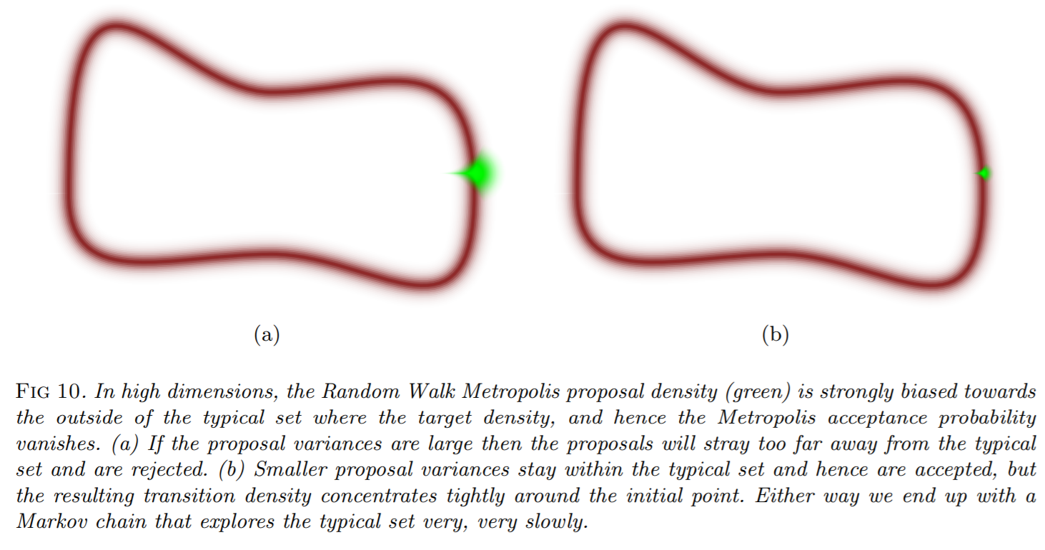
Recall that every single rejection is still evaluating the likelihood (since it's calculating an acceptance probability, finding it near zero, rejecting and starting again), and every likelihood call is calling our simulator, and so this is sllllllooooooooooooooowwwwwwwww in high dimensions!
What we need to do instead is ensure that we walk along the path of high probability. What we want to do is thus build a vector field that matches our high probability regions
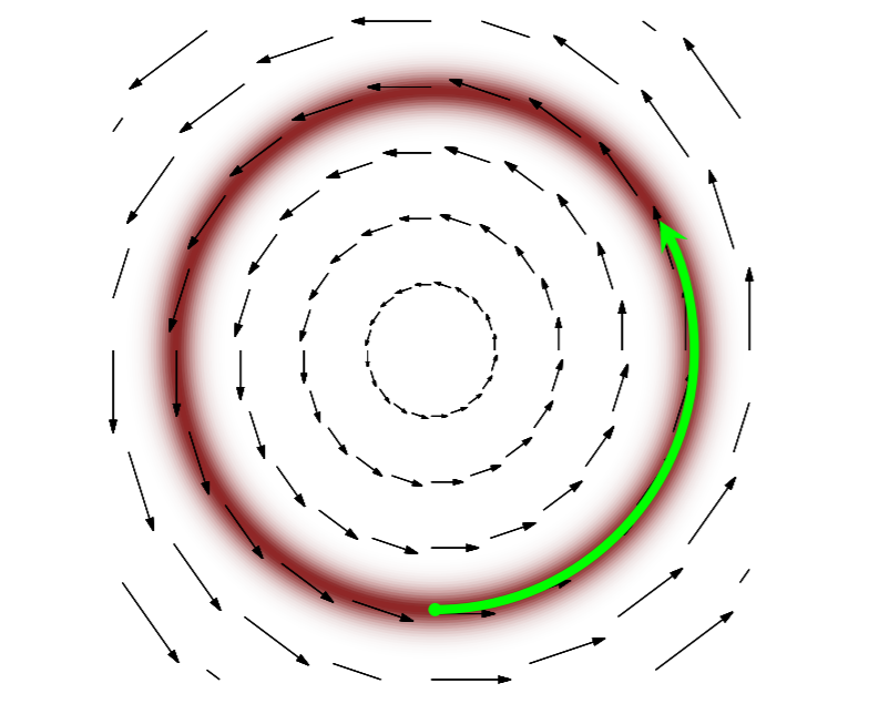
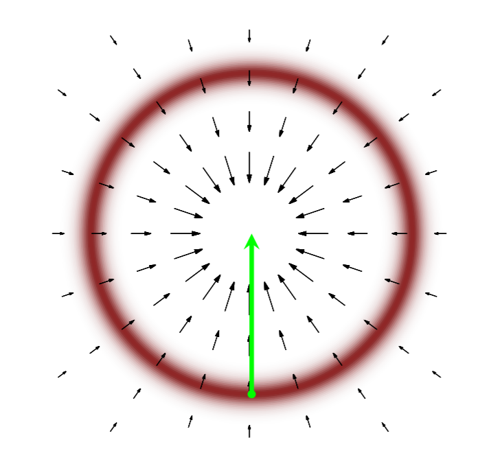
and follow said vector field (following a vector field is solving what kind of equation?). The first idea one might have is to use the gradient. However, while this idea has the right intentions, the issue is that the gradient of the probability will average out all of the possible probabilities, and will thus flow towards the mode of the distribution:
To overcome this issue, we look to physical systems and see that a satellite orbiting a planet always nicely stays on some manifold instead of following the gradient:
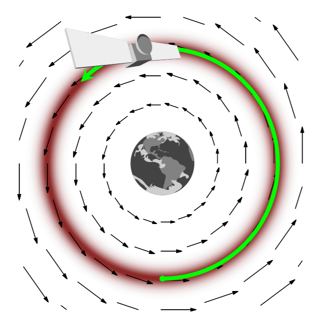
The reason why it does is because it has momentum. Recall from basic physics that one way to describe a physical system is through Hamiltonian mechanics, where $H(x,p)$ is the energy associated with the state $(x,p)$ (normally $x$ is location and $p$ is momentum). Due to conservation of energy, the solution of the dynamical equations leads to $H(x,p)$ being constant, and thus the dynamics follow the level sets of $H$. From the Hamiltonian the dynamics of the system are:
\[ \begin{align} \frac{dx}{dt} &= \frac{dH}{dp}\\ &= -\frac{dH}{dx} \end{align} \]
Here we want our Hamiltonian to be our posterior probability, so that way we stay on the manifold of high probability. This means:
\[ H(x,p) = - \log \pi(x,p) \]
where $\pi(x,p) = \pi(p|x)\pi(x)$ (where I am now using $pi$ for probability since $p$ is momentum!). So to lift from a probability over parameters to one that includes momentum, we simply need to choose a conditional distribution $\pi(p|x)$. This would mean that
\[ \begin{align} H(x,p) &= -\log \pi(p|x) - \log \pi(x)\\ &= K(p,x) + V(x) \end{align} \]
where $K$ is the kinetic energy and $V$ is the potential. Thus the potential energy is directly given by the posterior calculation, and the kinetic energy is thus a choice that is used to build the correct Hamiltonian. Hamiltonian Monte Carlo methods then dig into good ways to choose the kinetic energy function. This is done at the start (along with the choice of ODE solver time step) in such a way that it maximizes acceptance probabilities.
Connections to Differentiable Programming
\[ -\frac{dH}{dx} \]
requires calculating the gradient of the likelihood function with respect to the parameters, so we are once again using the gradient of our simulator! This means that all of our previous discussion on automatic differentiation and differentiable programming applies to the Hamiltonian Monte Carlo context.
There's another thread to follow that transformations of probability distributions are pushforwards of the Jacobian transformations (given the transformation of an integral formula), and this is used when doing variational inference.
Symplectic and Geometric Integration
One way to integrate the system of ODEs which result from the Hamiltonian system is to convert it to a system of first order ODEs and solve it directly. However, this loses information and can result in drift. This is demonstrated by looking at the long time solution of the pendulum:
using ParameterizedFunctions
u0 = [1.,0.]
harmonic! = @ode_def HarmonicOscillator begin
   dv = -x
   dx = v
end
tspan = (0.0,10.0)
tspan = (0.0,10000.0)
prob = ODEProblem(harmonic!,u0,tspan)
sol = solve(prob,Tsit5())
gr(fmt=:png) # Make it a PNG instead of an SVG since there's a lot of points!
plot(sol,idxs=(1,2))

plot(sol)

What is an oscillatory system slowly loses energy and falls inward towards the center. To avoid this issue, we can do a few things:
Project back to the manifold after steps. That can be costly (but almost might only need to happen every once in awhile!)
Use a symplectic integrator.
A symplectic integrator is an integrator who's solution lives on a symplectic manifold, i.e. it preserves area in in the $(x,p)$ ellipses as it numerically approximates the flow. This means that:
Long-time integrations are truly cyclic with only floating point drift.
Steps preserve area. In the sense of Hamiltonian Monte Carlo, this means preserve probability and thus increase the acceptance rate.
These properties are demonstrated in the Kepler problem demo. However, note that while the solution lives on a symplectic manifold, it isn't necessarily the correct symplectic manifold. The shift in the manifold is $\mathcal{O}(\Delta t^k)$ where $k$ is the order of the method. For more information on symplectic integration, consult this StackOverflow response which goes into depth.
Application: Bayesian Estimation of Differential Equation Parameters
For a full demo of probabilistic programming on a differential equation system, see this tutorial on Bayesian inference of pendulum parameters utilizing DifferentialEquations.jl and DiffEqBayes.jl.
Bayesian Estimation of Posterior Distributions with Variational Inference
Instead of using sampling, one can use variational inference to push through probability distributions. There are many ways to do variational inference, but a lot of the methods can be very model-specific. However, a recent change to probabilistic programming has been the development of Automatic Differentiation Variational Inference (ADVI): a general variational inference method which is not model-specific and instead uses AD. This has allowed for large expensive models to get effective distributional estimation, something that wasn't previously possible with HMC. In this section, we will build up this methodology and understand its performance characteristics.
ADVI as Optimization
In this form of variational inference, we wish to directly estimate the posterior distribution. To do so, we pick a functional form to represent the solution $q(\theta; \phi)$ where $\phi$ are latent variables. We want our resulting distribution to fit the posterior, and thus we enforce that:
\[ \phi^\ast = \text{argmin}_{\phi} \text{KL} \left(q(\theta; \phi) \Vert p(\theta | D)\right) \]
where KL is the KL-divergence. KL-divergence is a distance function over probability distributions, and so this is simply a cost function over the distance between a chosen distribution and a desired distribution, where when $\phi$ are good we will have $q$ as a good approximation to the posterior.
However, the KL divergence lacks an analytical form because it requires knowing the posterior, the quantity we are trying to numerically estimate. However, it turns out that we can instead maximize the Evidence Lower Bound (ELBO):
\[ \mathcal{L}(\phi) = \mathbb{E}_{q}[\log p(x,\theta)] - \mathbb{E}_q [\log q(\theta; \phi)] \]
The ELBO is equivalent to the negative KL divergence up to a constant $\log p(x)$, which means that maximizing this is equivalent to minimizing the KL divergence.
One last detail is necessary in order for this problem to be tractable. To know the set of possible values to optimize over, we assume that the support of $q$ is a subset of the support of the prior. This means that our prior has to cover the probability distribution, which makes sense and matches Cromwell's rule for MCMC.
At this point, we now assume that $q$ is Gaussian. When we rewrite the ELBO in terms of the standard Gaussian, we receive an expectation that is automatically differentiable. Calculating gradients is thus done with AD. Using only one or a few solves gives a noisy gradient to sample and optimize the latent variables to hone in on latent variables.
A Note on Implementation of Optimization for Probabilistic Programming
Variable domains can be constrained. For example, you may require a positive value. This can be handled by a transformation. For example, if $y$ must be positive, then one can optimize implicitly using $\exp(y)$ at every point, this allowing $y$ to be any real value with then $\exp(y)$ is positive. This turns the problem into an unconstrained optimization over the real numbers, and similar transformations can be done with any of the standard probability distribution's support function.
Citation
For Hamiltonian Monte Carlo, the images were taken from A Conceptual Introduction to Hamiltonian Monte Carlo by Michael Betancourt.