Code Profiling and Optimization
Chris Rackauckas
December 11th, 2020
Youtube Video
This is just a quick look into code profiling. By now we should be writing high performance parallel code which is combining machine learning and scientific computing techniques and doing large-scale parameter analyses on the models. However, at this point it may be difficult to understand where our performance difficulties lie. This is where we turn to code profiling tooling.
Type Inference Checking
The most common way for code to slow down is via type-inference issues. One can normally work through them by "thinking like a compiler" and seeing what would be inferable. For example, a common issue is to not concretely type one's types. For example:
struct MyStruct
  a::AbstractArray
end
x = MyStruct([1,2,3])
function f(x)
  x.a[1]
end
using InteractiveUtils
@code_warntype f(x)
MethodInstance for f(::MyStruct)
  from f(x) @ Main ~/work/SciMLBook/SciMLBook/_weave/lecture18/code_profili
ng.jmd:6
Arguments
  #self#::Core.Const(Main.f)
  x::MyStruct
Body::ANY
1 ─ %1 = Base.getproperty(x, :a)::ABSTRACTARRAY
│   %2 = Base.getindex(%1, 1)::ANY
└──      return %2
In this case, the return type is not inferred and using MyStruct will generate slow code. The reason for this is quite simple: x.a can only be inferred as AbstractArray, and thus the element type x.a[1] and the exact dispatch cannot be known until the function finds out at runtime what kind of array it is. As a result, the compiler throws the only thing it can: it puts Any as the inferred type and runs slow code.
We can instead utilize a concrete struct or use a parametric type to create a family of related structs:
struct MyStruct2{A <: AbstractArray}
  a::A
end
x2 = MyStruct2([1,2,3])
@code_warntype f(x2)
MethodInstance for f(::MyStruct2{Vector{Int64}})
  from f(x) @ Main ~/work/SciMLBook/SciMLBook/_weave/lecture18/code_profili
ng.jmd:6
Arguments
  #self#::Core.Const(Main.f)
  x::MyStruct2{Vector{Int64}}
Body::Int64
1 ─ %1 = Base.getproperty(x, :a)::Vector{Int64}
│   %2 = Base.getindex(%1, 1)::Int64
└──      return %2
and now it's inferred because the information that it would need is inferrable.
But what if we needed help? The first tool of course is @code_warntype. But for deeper functions you may want more tooling. A nice tool is JET.jl which statically analyzes your code and reports type instabilities. In our example we see:
using JET
@report_opt f(x)
which points out our first problem is getting the untyped array out of the MyStruct. On larger functions it can do even more:
function naive_sum(xs)
  s = 0
  for x in xs
    s += x
  end
  return s
end
@report_opt naive_sum([1.])
and alert you to multiple lines which are causing problems.
However, for even larger functions you can still have many issues that are hard to dig into with Julia a linear tool. For thus, Cthulhu.jl's @descend macro lets you interactively dig into the function to find the problematic lines. For the best introduction, watch Valentin Churavy's JuliaCon 2019 talk
Flame Graphs
Flame graphs are a common tool for illustrating performance. To demonstrate this let's look at the solution to an ODE from DifferentialEquations.jl's OrdinaryDiffEq.jl. The code is the following:
using OrdinaryDiffEq
function lorenz(du,u,p,t)
 du[1] = 10.0(u[2]-u[1])
 du[2] = u[1]*(28.0-u[3]) - u[2]
 du[3] = u[1]*u[2] - (8/3)*u[3]
end
u0 = [1.0;0.0;0.0]
tspan = (0.0,100.0)
prob = ODEProblem(lorenz,u0,tspan)
sol = solve(prob,Tsit5())
using Plots; plot(sol,idxs=(1,2,3))

To generate the flame graph, first we want to create a profile. To do this we will use the Profile module's @profile. Note that a profile should be "sufficiently large", so on quick functions you may want to run the code plenty of times. Make sure the profile does not include compilation if you want good results!
sol = solve(prob,Tsit5())

using Profile
@profile for i in 1:1000 sol = solve(prob,Tsit5()) end
This profiler is a statistical or sampling profiler, which means it periodically samples where it is at in a code and thus understands the hotspots in the code by tallying how many samples are in a certain area. We can first visualize this by printing it out:
#Profile.print()
However, that printout can often times be hard to read. Instead, we can visualize it with a flame graph. Using VSCode with the Julia extension, open the command palette and run Julia: Show Profile. Alternatively, use ProfileView.jl:
using ProfileView
ProfileView.view()
(PProf.jl exports to Google PProf which has many more features than ProfileView.jl)
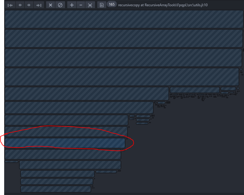
Each block corresponds to a function call. The horizontal length is the amount of time spent in that function, while the vertical grouping is for call nesting, i.e. you are below the function that called you. The portion that is circled is where the mouse pointer was at, and while hovering over this it said what function it corresponded to: recursivecopy in RecursiveArrayTools.jl. If we click on this, it sends us to the hotspot:
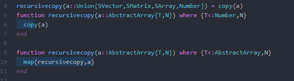
The flame graph gives you a visual indicator of how much time is spent at a given line. Here we see that most of the time is spent inside of the map operation which calls recursivecopy on the elements, which then does copy(a).
This tells us that the main cost of our code is the part that is copying the arrays to save them! Thus let's generate a new profile where the ODE solver saves less:
Profile.clear()
sol = solve(prob,Tsit5(),save_everystep=false)

@profile for i in 1:1000 sol = solve(prob,Tsit5(),save_everystep=false) end
using ProfileView
ProfileView.view()
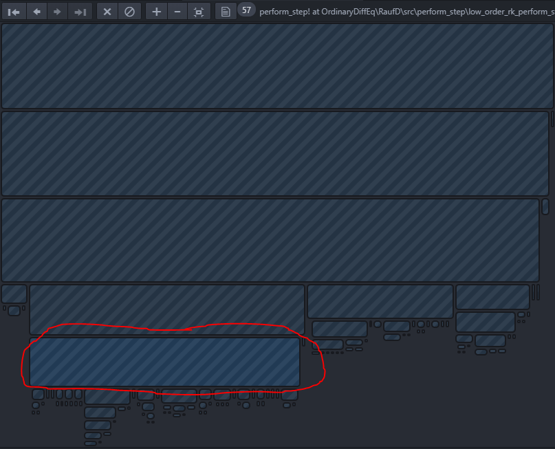
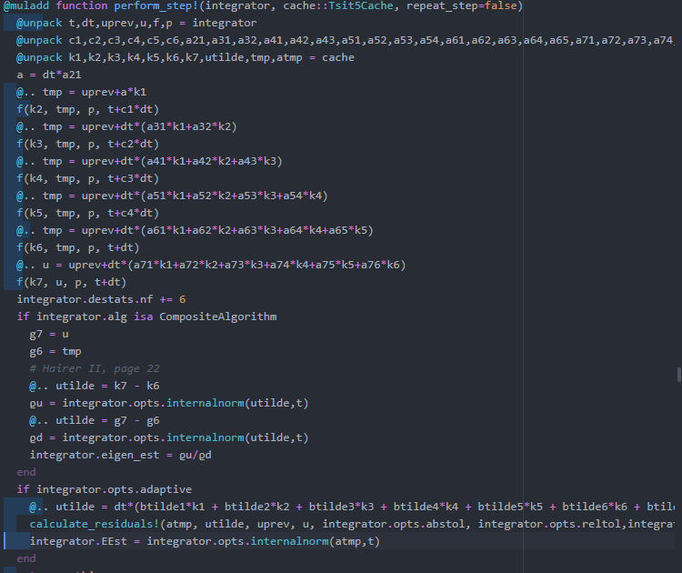
Now we see that the majority of the time is spent in the perform_step! method, which is:
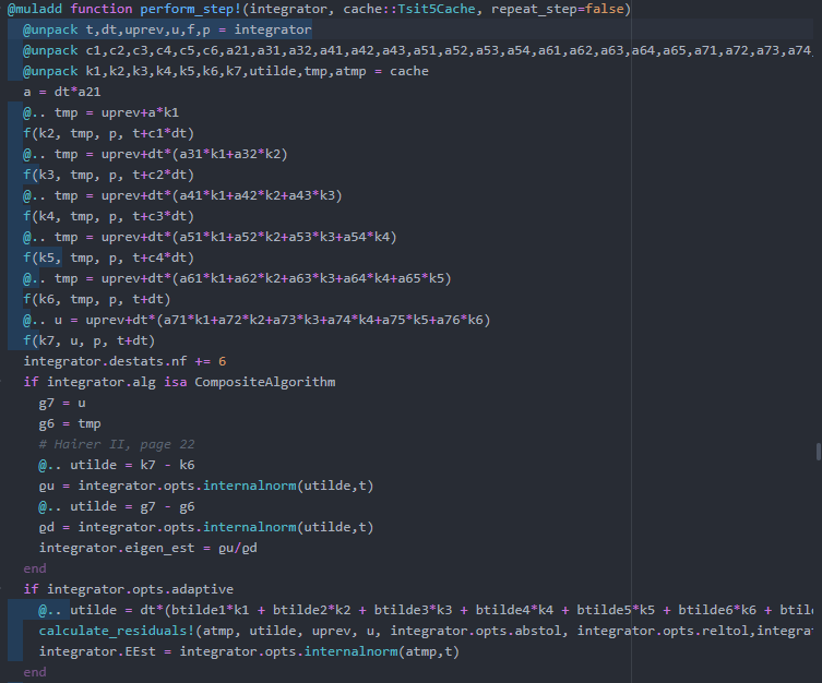
We can notice that there is still quite a bit of jitter in the profile since each of the f calls here should be exactly the same length, but upping the number of solves in the loop would help with that:
@profile for i in 1:10000 sol = solve(prob,Tsit5(),save_everystep=false) end
using ProfileView
ProfileView.view()
Now that this looks like a fairly good profile, we can use this to dig in and find out what lines need to be optimized!