Uncertainty Programming, Generalized Uncertainty Quantification
Chris Rackauckas
December 12th, 2020
Youtube Video
In this lecture we will mix two separate topics: uncertainty quantification and adaptivity of algorithms. Using compiler-based tooling, similar to how automatic differentiation and probabilistic programming toolchains, we will show how one can begin to pushforward uncertainties of a model or calculation. This leads to an idea of uncertainty programming, a term which is not in use but should be justified by these notes.
What is Uncertainty Quantification?
Uncertainty quantification is the identification and quantification of sources of uncertainty. In our training of a neural differential equation, we have seen that the question of uncertainty can quickly become muddled. Results are inexact because of:
Truncation errors in the ODE solve
Truncation errors in the adjoint ODE solve
Truncation errors in the interpolation calculation
Numerical errors in every dot product along the way (!)
Numerical errors in matrix multiplication and linear solving (latter when implicit)
Numerical errors in backpropagation
Measurement errors in our fitting data
Randomness in the optimizer (when stochastic, like ADAM)
What is the error in the model specification / model form?
"How correct is my model?" is thus a very involved question, since you'd have to know that every source of uncertainty is contained. In some cases we have rigorous mathematical results proving bounds. In other cases, we need to find empirical ways to quantify what's going on using our known bounds.
Some High Level UQ Techniques
Two high level UQ techniques fall out of methodologies we have recently discussed. If we fit a model $f$ to data, be it a neural network, a neural ODE, or some physical ODE model, we can fit it probabilistically using the Bayesian estimation or probabilistic programming tools previously described. With this form of fitting, one can ask the question "what are the likely results from the model given these parameter distributions?", which can then be answered through Monte Carlo sampling.
Another form of high level UQ is global sensitivity analysis, which gives a measurement for how much the output is going to vary over a wide range and thus relates uncertainties in the input to uncertainties in the output.
Pushforward Methods for Uncertainties
Instead of relying on expensive Monte Carlo methods for the pushforward of an uncertainty, we can derive a more programmatic approach to uncertainty quantification through the use of uncertain number arithmetic.
To start, let's first revive the old physics way to doing simple uncertainty quantification. If you have two numbers, $x = a \pm b$, one might remember the rules like,
\[ \alpha + a = (\alpha + a) \pm b \]
\[ \alpha a = \alpha a \pm |\alpha| b \]
Let's investigate this a bit more and see if we can develop an arithmetic, like dual numbers, to then propagate through whole programs. This idea comes from the arithmetic on normally distributed random variables. If we interpret $x \sim N(a,b)$, i.e. a normally distributed random variable with mean $a$ and standard deviation $b$, then the distributions follow that:
\[ \alpha + a \sim N(\alpha + a,b) \]
\[ \alpha a \sim N(\alpha a,|\alpha|b) \]
From here we can begin to expand to multiple variables. If $f = Ax$ where $x ~ N(\mu,\Sigma)$ is a multidimensional random variable, then
\[ E[f] = A\mu \]
and
\[ V[f] = A \Sigma A^T \]
Now take a nonlinear $f(x)$. By a Taylor expansion we have that
\[ f(x) = f_0 + Jx + \ldots \]
i.e. the linear approximation is $f_0 + Jx$ where $f_0 = f(\mu)$ and $J$ is the Jacobian matrix. If we do a pushforward on the linear approximation, we receive
\[ f(x) ~ N(f(\mu),J\Sigma J^T) \]
which gives the rules for the pushforward on any possible function through the linearization. But the linearization is the same as the forward differencing ones, meaning that we can augment existing tooling for forward-mode automatic differentiation to perform pushforwards of uncertain quantities. A library which does this is Measurements.jl. Note that this library additionally tracks the correlations between each variable so that the second order terms are accurate.
Measurements.jl in Practice: Measurements on DifferentialEquations
Since DifferentialEquations.jl takes in arbitrary number types, we can have it recompile to do the arithmetics of uncertainty propagation. For example, the following solves the pendulum of arbitrary amplitude with respect to uncertain parameters and initial conditions:
\[ \ddot{\theta} + \frac{g}{L} \sin(\theta) = 0 \]
using OrdinaryDiffEq, OrdinaryDiffEqLowOrderRK, Measurements
gaccel = 9.79 ± 0.02; # Gravitational constants
L = 1.00 ± 0.01; # Length of the pendulum

#Initial Conditions
u₀ = [0 ± 0, π / 3 ± 0.02] # Initial speed and initial angle
tspan = (0.0, 6.3)

#Define the problem
function simplependulum(du,u,p,t)
    θ  = u[1]
    dθ = u[2]
    du[1] = dθ
    du[2] = -(gaccel/L) * sin(θ)
end

#Pass to solvers
prob = ODEProblem(simplependulum, u₀, tspan)
sol = solve(prob, Tsit5(), reltol = 1e-6)

using Plots
plot(sol,plotdensity=100,idxs=2)

From here it is clear that as the pendulum goes forward, the uncertainty grows since the exact period is unclear. Notice another nice feature is on display here: the Plots.jl Recipe System. The plotting just worked because the recipes are a type-recursive system. The three steps were:
The DifferentialEquations solution recipe transformed the ODE solution into an array of measurement variables
The Measurements recipe transformed the measurement variables into an array of floats along with a series of error bars
This array of floats was recognized as a native format, and thus the plot was made.
Note that this idea of discretizing distributions and pushing them through a full calculation can be done with more accuracy by using things like orthogonal polynomial expansions. This is the polynomial chaos expansion approach which we will not cover, but there is a PolyChaos.jl package one can explore.
Quantifying Numerical Uncertainty with Intervals
While Measurements gives a sense of uncertainty quantification for unknown inputs, a different form of uncertainty quantification is that for floating point uncertainties. For example, when you calculate $sin(2.3)$ on your computer, this has an error in the approximation, and what if we wanted to push these errors forward to get an interval which bounds the possible values given the numerical uncertainty? This is done via interval arithmetic.
For this we can use IntervalArithmetic.jl. The idea of interval arithmetic is to work rigorously on sets of real numbers, i.e.
\[ [a,b] = \{x\in\mathbb{R} : a\leq x \leq b\} \]
We can construct an interval given the interval method:
using IntervalArithmetic
x = interval(0.1,0.2)
[0.1, 0.2]_com
Here the operator catches the constants at compile time and notices that 0.1 and 0.2 cannot be exactly represented in floating point numbers, and thus on the left side it rounds down by one floating point number and on the right it rounds up by one floating point number to make sure the set rigorously contains the correct value.
From here, non-monotone functions can propagate intervals like:
[a, b]^2 := [a^2, b^2]  if 0 < a < b
          = [0, max(a^2, b^2)]  if a < 0 < b
          = [b^2, a^2] if a < b < 0
The rules can get fairly complicated and may need to be derived for each individual elementary function, but, just like automatic differentiation, recursion can be performed to get to a bottom of primitives which is known to then propagate forward the intervals.
Because this form of uncertainty quantification is rigorous, we can prove theorem on it. For example, let's say we want to show that
h(x) = x^2 - 2
h (generic function with 3 methods)
has no roots in $[3,4]$. Since these are rigorous bounds, it holds that
h(interval(3,4))
[7.0, 14.0]_com_NG
is a rigorous bound on the possible values, and thus it must not have a root in this interval.
Problems with Interval Arithmetic
Interval arithmetic is nice... but it can have some issues. It's rigorous but it's also conservative, meaning that the intervals can be much larger than one would expect given the actual uncertainties seen in practice. One phenomena which causes this can be seen by looking at that pendulum:
gaccel = interval(9.77,9.81); # Gravitational constants
L = interval(0.99,1.01); # Length of the pendulum

#Initial Conditions
u₀ = [interval(0,0), interval(((π / 3.0)-0.02),((π / 3.0)+0.02))] # Initial speed and initial angle
tspan = (0.0, 6.3)

#Define the problem
function simplependulum(du,u,p,t)
    θ  = u[1]
    dθ = u[2]
    du[1] = dθ
    du[2] = -(gaccel/L) * sin(θ)
end

#Pass to solvers
prob = ODEProblem(simplependulum, u₀, tspan)
sol = solve(prob, Euler(), dt=0.1)
retcode: Success
Interpolation: 3rd order Hermite
t: 64-element Vector{Float64}:
 0.0
 0.1
 0.2
 0.30000000000000004
 0.4
 0.5
 0.6
 0.7
 0.7999999999999999
 0.8999999999999999
 ⋮
 5.4999999999999964
 5.599999999999996
 5.699999999999996
 5.799999999999995
 5.899999999999995
 5.999999999999995
 6.099999999999994
 6.199999999999994
 6.3
u: 64-element Vector{Vector{Interval{Float64}}}:
 [[0.0, 0.0]_com, [1.02719, 1.0672]_com]
 [[0.102719, 0.10672]_com_NG, [1.02719, 1.0672]_com_NG]
 [[0.205439, 0.21344]_com_NG, [0.921648, 0.968009]_com_NG]
 [[0.297604, 0.310241]_com_NG, [0.711751, 0.770677]_com_NG]
 [[0.368779, 0.387309]_com_NG, [0.409239, 0.487027]_com_NG]
 [[0.409703, 0.436011]_com_NG, [0.0349758, 0.138328]_com_NG]
 [[0.413201, 0.449844]_com_NG, [-0.383512, -0.246995]_com_NG]
 [[0.374849, 0.425144]_com_NG, [-0.814384, -0.635418]_com_NG]
 [[0.293411, 0.361603]_com_NG, [-1.22309, -0.989588]_com_NG]
 [[0.171103, 0.262644]_com_NG, [-1.57365, -1.26935]_com_NG]
 ⋮
 [[-58.9404, 74.8546]_com_NG, [-34.3214, 39.0545]_com_NG]
 [[-62.3725, 78.76]_com_NG, [-35.3124, 40.0454]_com_NG]
 [[-65.9037, 82.7646]_com_NG, [-36.3033, 41.0363]_com_NG]
 [[-69.5341, 86.8682]_com_NG, [-37.2942, 42.0272]_com_NG]
 [[-73.2635, 91.0709]_com_NG, [-38.2851, 43.0181]_com_NG]
 [[-77.092, 95.3727]_com_NG, [-39.276, 44.0091]_com_NG]
 [[-81.0196, 99.7736]_com_NG, [-40.2669, 45.0]_com_NG]
 [[-85.0462, 104.274]_com_NG, [-41.2578, 45.9909]_com_NG]
 [[-89.172, 108.873]_com_NG, [-42.2487, 46.9818]_com_NG]
While we start out with reasonably small intervals, it turns out that every operation is calculating "what is the largest I could be? What is the smallest I could be?". Comparing these extremes at every operation means that, yes, by the end, given the uncertainty in the period, the solution lies in the interval $[-11642.4,11652.2]$, but that's not a particularly helpful estimate! This demonstrates the exponential explosion of interval estimates.
But note that part of why it got so large is because we started with "such large" intervals. If we only used this to measure the uncertainty of the floating point arithmetic, then the intervals are much better contained:
gaccel = interval(9.8,9.8); # Gravitational constants
L = interval(1.0,1.0); # Length of the pendulum

#Initial Conditions
u₀ = [interval(0,0), interval((π / 3.0),(π / 3.0))] # Initial speed and initial angle
tspan = (0.0, 6.3)

#Define the problem
function simplependulum(du,u,p,t)
    θ  = u[1]
    dθ = u[2]
    du[1] = dθ
    du[2] = -(gaccel/L) * sin(θ)
end

#Pass to solvers
prob = ODEProblem(simplependulum, u₀, tspan)
sol = solve(prob, Euler(), dt=0.001)
retcode: Success
Interpolation: 3rd order Hermite
t: 6301-element Vector{Float64}:
 0.0
 0.001
 0.002
 0.003
 0.004
 0.005
 0.006
 0.007
 0.008
 0.009000000000000001
 ⋮
 6.292000000000436
 6.293000000000436
 6.294000000000437
 6.295000000000437
 6.296000000000437
 6.297000000000438
 6.298000000000438
 6.299000000000438
 6.3
u: 6301-element Vector{Vector{Interval{Float64}}}:
 [[0.0, 0.0]_com, [1.04719, 1.0472]_com]
 [[0.00104719, 0.0010472]_com_NG, [1.04719, 1.0472]_com_NG]
 [[0.00209439, 0.0020944]_com_NG, [1.04718, 1.04719]_com_NG]
 [[0.00314158, 0.00314159]_com_NG, [1.04716, 1.04717]_com_NG]
 [[0.00418874, 0.00418875]_com_NG, [1.04713, 1.04714]_com_NG]
 [[0.00523588, 0.00523589]_com_NG, [1.04709, 1.0471]_com_NG]
 [[0.00628298, 0.00628299]_com_NG, [1.04704, 1.04705]_com_NG]
 [[0.00733002, 0.00733003]_com_NG, [1.04698, 1.04699]_com_NG]
 [[0.008377, 0.00837701]_com_NG, [1.04691, 1.04692]_com_NG]
 [[0.00942391, 0.00942392]_com_NG, [1.04682, 1.04683]_com_NG]
 ⋮
 [[0.224664, 0.224668]_com_NG, [0.82007, 0.820081]_com_NG]
 [[0.225484, 0.225488]_com_NG, [0.817887, 0.817897]_com_NG]
 [[0.226302, 0.226306]_com_NG, [0.815696, 0.815706]_com_NG]
 [[0.227117, 0.227121]_com_NG, [0.813497, 0.813508]_com_NG]
 [[0.227931, 0.227935]_com_NG, [0.81129, 0.811301]_com_NG]
 [[0.228742, 0.228746]_com_NG, [0.809076, 0.809086]_com_NG]
 [[0.229551, 0.229555]_com_NG, [0.806854, 0.806864]_com_NG]
 [[0.230358, 0.230362]_com_NG, [0.804624, 0.804634]_com_NG]
 [[0.231163, 0.231167]_com_NG, [0.802386, 0.802397]_com_NG]
Contextual Uncertainty Quantification
Those previous methods were non-contextual and worked directly through program modification. However, by not "clumping" interactions, uncertainty quantification can have overestimates like is seen with the interval growth. Thus, just like with reverse-mode AD, can we instead look for higher order uncertainty primitives on which to build such a system? When digging into reverse-mode AD, we saw that adjoint problems in engineering corresponded to the the reverse-mode rules for things like linear solve, eigenvalue problems, and the solution of ODEs. There does not seem to be a general analogue in the case of uncertainty quantification, but there is hope. Since this is a big enough field, people have found special cases where uncertainty can be quantified in interesting manners. Let's look specifically at ODEs.
Quantifying Uncertainty in ODE Solves for Adaptivity
However, in some sense, adaptive numerical methods work by embedding a form of uncertainty quantification. Let's take a look at the Bogaki-Shampine method for solving ODEs:
Notice that there's a $y_{n+1}$ and a $z_{n+1}$ for two separate solutions for the next time step. It so happens that $y$ is $\mathcal{O}(\Delta t^3)$ while $z$ is $\mathcal{O}(\Delta t^2)$, meaning that $E = z_{n+1} - y_{n+1}$ is a $\mathcal{O}(\Delta t^2)$ estimate for the error in a given step, since the two must both be "$\Delta t^2$ close enough" to the true solution. Similarly, when we looked at the Dormand-Prince method in our homework, the tableau:
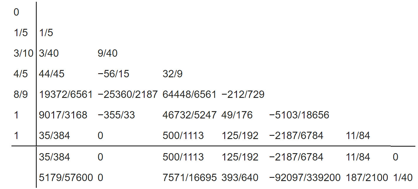
had a second row as well, with the first being $\mathcal{O}(n^5)$ and the second being $\mathcal{O}(n^4)$. Thus these Runge-Kutta methods naturally have error estimators. In standard usage, they are compared to the tolerances, like:
\[ q = \frac{E}{\text{reltol}\max(z_n,z_{n+1}) + \text{abstol}} \]
and when $q<1$, the $\Delta t$ gives an error larger than the tolerances and so the step is rejected, decreased, and tried again. In many cases, one may control the error proportionally to this error estimator, i.e. the next $\Delta t$ is the product $q \Delta t$.
That's all for adapting to a tolerance, but can we use this to propagate uncertainties? It turns out we can. This is known as the ProbInts method. Essentially, instead of an ODE, we can think of having solved a stochastic differential equation whose additive noise term of size which matches our error estimate. Specifically, adding a noise which is normally distributed with mean zero and standard deviation $(\Delta t)^{p}$, where $p$ is the order of the adaptive error estimate (i.e. the order of the lower approximation), is an approximation to the possible values that could have occurred given the noise that was seen. By adding this at every step, we can then recover a distribution of possible solutions/trajectories.
ProbInts in Action
using DiffEqCallbacks
function fitz(du,u,p,t)
  V,R = u
  a,b,c = p
  du[1] = c*(V - V^3/3 + R)
  du[2] = -(1/c)*(V -  a - b*R)
end
u0 = [-1.0;1.0]
tspan = (0.0,20.0)
p = (0.2,0.2,3.0)
prob = ODEProblem(fitz,u0,tspan,p)

cb = AdaptiveProbIntsUncertainty(5) # 5th order method
sol = solve(prob,Tsit5())
ensemble_prob = EnsembleProblem(prob)
sim = solve(ensemble_prob,Tsit5(),trajectories=100,callback=cb)
plot(sim,idxs=(0,1),linealpha=0.4)

cb = AdaptiveProbIntsUncertainty(5)
sol = solve(prob,Tsit5())
ensemble_prob = EnsembleProblem(prob)
sim = solve(ensemble_prob,Tsit5(),trajectories=100,callback=cb,abstol=1e-3,reltol=1e-1)
plot(sim,idxs=(0,1),linealpha=0.4)

Notice that while an interval estimate would have grown to allow all extremes together, this form keeps the trajectories alive, allowing them to fall back to the mode, which decreases the true uncertainty. This is thus a good explanation as to why general methods will overestimate uncertainty.
Adjoints of Uncertainty and the Koopman Operator
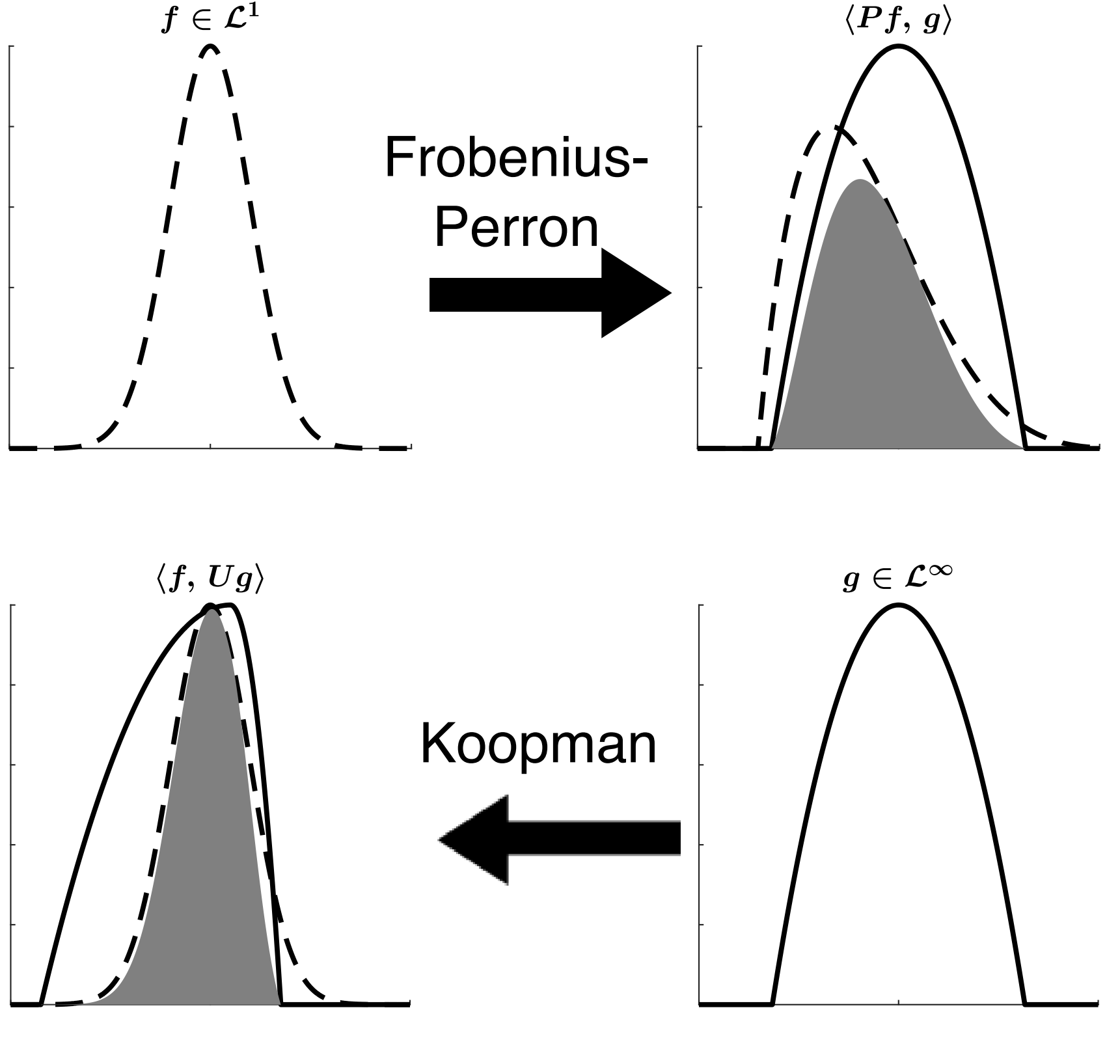
Everything that we've demonstrated here so far can be thought of as "forward mode uncertainty quantification". For every example we have constructed a method such that, for a known probability distribution in x, we build the probability distribution of the output of the program, and then compute quantities from that. On a dynamical system this pushforward of a measure is denoted by the Frobenius-Perron operator. With a pushforward operator $P$ and an initial uncertainty density $f$, we can represent calculating the expected value of some cost function on the solution via:
\[ \mathbb{E}[g(x)|X \sim Pf] = \int_{S(A)} P f(x) g(x) dx \]
where $S$ is the program, i.e. $S(A)$ is the total set of points by pushing every value of $A$ through our program, and $P f(x)$ is the pushforward operator applied to the probability distribution. What this means is that, to calculate the expectation on the output of our program, like to calculate the mean value of the ODE's solution given uncertainty in the parameters, we can pushforward the probability distribution to construct $Pf$ and on this probability distribution calculate the expected value of some $g$ cost function on the solution.
The problem, as seen earlier, is that pushing forward entire probability distributions is a fairly expensive process. We can instead think about doing the adjoint to this cost function, i.e. pulling back the cost function and computing it on the initial density. In terms of inner product notation, this would be doing:
\[ \langle Pf,g \rangle = \langle f, Ug \rangle \]
meaning $U$ is the adjoint operator to the pushforward $P$. This operator is known as the Koopman operator. There are many properties one can use about the Koopman operator, one special property being it's a linear operator on the space of observables, but it also gives a nice expression for computing uncertainty expectations. Using the Koopman operator, we can rewrite the expectation as:
\[ \mathbb{E}[g(x)|X \sim Pf] = \mathbb{E}[Ug(x)|X \sim f] \]
or perform the integral on the pullback of the cost function, i.e.
\[ \mathbb{E}[g(x)|X \sim f] = \int_A Ug(x) f(x) dx \]
In images it looks like:
This expression gives us a fast way to compute expectations on the program output without having to compute the full uncertainty distribution on the output. This can thus be used for optimization under uncertainty, i.e. the optimization of loss functions with respect to expectations of the program's output under the assumption of given input uncertainty distributions. For more information, see The Koopman Expectation: An Operator Theoretic Method for Efficient Analysis and Optimization of Uncertain Hybrid Dynamical Systems.